Generalized coordinates

Last updated

In analytical mechanics, generalized coordinates are a set of parameters used to represent the state of a system in a configuration space. These parameters must uniquely define the configuration of the system relative to a reference state. [1] The generalized velocities are the time derivatives of the generalized coordinates of the system. The adjective "generalized" distinguishes these parameters from the traditional use of the term "coordinate" to refer to Cartesian coordinates.

Contents

An example of a generalized coordinate would be to describe the position of a pendulum using the angle of the pendulum relative to vertical, rather than by the x and y position of the pendulum.

Although there may be many possible choices for generalized coordinates for a physical system, they are generally selected to simplify calculations, such as the solution of the equations of motion for the system. If the coordinates are independent of one another, the number of independent generalized coordinates is defined by the number of degrees of freedom of the system. [2] [3]

Generalized coordinates are paired with generalized momenta to provide canonical coordinates on phase space.

Constraints and degrees of freedom

Generalized coordinates open straight path 2d 1df.svg
Open straight path
Generalized coordinates open curved path 2d 1df.svg
Open curved path F(x, y) = 0
Generalized coordinates closed path 2d 1df.svg
Closed curved path C(x, y) = 0
One generalized coordinate (one degree of freedom) on paths in 2D. Only one generalized coordinate is needed to uniquely specify positions on the curve. In these examples, that variable is either arc length s or angle θ. Having both of the Cartesian coordinates (x, y) are unnecessary since either x or y is related to the other by the equations of the curves. They can also be parameterized by s or θ.
Non generalized coordinates open curved path 2d 1df.svg
Open curved path F(x, y) = 0. Multiple intersections of radius with path.
Non generalized coordinates closed curved path 2d 1df.svg
Closed curved path C(x, y) = 0. Self-intersection of path.
The arc length s along the curve is a legitimate generalized coordinate since the position is uniquely determined, but the angle θ is not since there are multiple positions for a single value of θ.

Generalized coordinates are usually selected to provide the minimum number of independent coordinates that define the configuration of a system, which simplifies the formulation of Lagrange's equations of motion. However, it can also occur that a useful set of generalized coordinates may be dependent, which means that they are related by one or more constraint equations.

Holonomic constraints

Generalized coordinates open curved path 3d 2df.svg
Open curved surface F(x, y, z) = 0
Generalized coordinates closed curved path 3d 2df.svg
Closed curved surface S(x, y, z) = 0
Two generalized coordinates, two degrees of freedom, on curved surfaces in 3D. Only two numbers (u, v) are needed to specify the points on the curve, one possibility is shown for each case. The full three Cartesian coordinates (x, y, z) are not necessary because any two determines the third according to the equations of the curves.

For a system of N particles in 3D real coordinate space, the position vector of each particle can be written as a 3-tuple in Cartesian coordinates:

Any of the position vectors can be denoted rk where k = 1, 2, …, N labels the particles. A holonomic constraint is a constraint equation of the form for particle k [4] [lower-alpha 1]

which connects all the 3 spatial coordinates of that particle together, so they are not independent. The constraint may change with time, so time t will appear explicitly in the constraint equations. At any instant of time, any one coordinate will be determined from the other coordinates, e.g. if xk and zk are given, then so is yk. One constraint equation counts as one constraint. If there are C constraints, each has an equation, so there will be C constraint equations. There is not necessarily one constraint equation for each particle, and if there are no constraints on the system then there are no constraint equations.

So far, the configuration of the system is defined by 3N quantities, but C coordinates can be eliminated, one coordinate from each constraint equation. The number of independent coordinates is n = 3NC. (In D dimensions, the original configuration would need ND coordinates, and the reduction by constraints means n = NDC). It is ideal to use the minimum number of coordinates needed to define the configuration of the entire system, while taking advantage of the constraints on the system. These quantities are known as generalized coordinates in this context, denoted qj(t). It is convenient to collect them into an n-tuple

which is a point in the configuration space of the system. They are all independent of one other, and each is a function of time. Geometrically they can be lengths along straight lines, or arc lengths along curves, or angles; not necessarily Cartesian coordinates or other standard orthogonal coordinates. There is one for each degree of freedom, so the number of generalized coordinates equals the number of degrees of freedom, n. A degree of freedom corresponds to one quantity that changes the configuration of the system, for example the angle of a pendulum, or the arc length traversed by a bead along a wire.

If it is possible to find from the constraints as many independent variables as there are degrees of freedom, these can be used as generalized coordinates. [5] The position vector rk of particle k is a function of all the n generalized coordinates (and, through them, of time), [6] [7] [8] [5] [nb 1]

and the generalized coordinates can be thought of as parameters associated with the constraint.

The corresponding time derivatives of q are the generalized velocities,

(each dot over a quantity indicates one time derivative). The velocity vector vk is the total derivative of rk with respect to time

and so generally depends on the generalized velocities and coordinates. Since we are free to specify the initial values of the generalized coordinates and velocities separately, the generalized coordinates qj and velocities dqj/dt can be treated as independent variables.

Non-holonomic constraints

A mechanical system can involve constraints on both the generalized coordinates and their derivatives. Constraints of this type are known as non-holonomic. First-order non-holonomic constraints have the form

An example of such a constraint is a rolling wheel or knife-edge that constrains the direction of the velocity vector. Non-holonomic constraints can also involve next-order derivatives such as generalized accelerations.

Physical quantities in generalized coordinates

Kinetic energy

The total kinetic energy of the system is the energy of the system's motion, defined as [9]

in which · is the dot product. The kinetic energy is a function only of the velocities vk, not the coordinates rk themselves. By contrast an important observation is [10]

which illustrates the kinetic energy is in general a function of the generalized velocities, coordinates, and time if the constraints also vary with time, so T = T(q, dq/dt, t).

In the case the constraints on the particles are time-independent, then all partial derivatives with respect to time are zero, and the kinetic energy is a homogeneous function of degree 2 in the generalized velocities.

Still for the time-independent case, this expression is equivalent to taking the line element squared of the trajectory for particle k,

and dividing by the square differential in time, dt2, to obtain the velocity squared of particle k. Thus for time-independent constraints it is sufficient to know the line element to quickly obtain the kinetic energy of particles and hence the Lagrangian. [11]

It is instructive to see the various cases of polar coordinates in 2D and 3D, owing to their frequent appearance. In 2D polar coordinates (r, θ),

in 3D cylindrical coordinates (r, θ, z),

in 3D spherical coordinates (r, θ, φ),

Generalized momentum

The generalized momentum "canonically conjugate to" the coordinate qi is defined by

If the Lagrangian L does not depend on some coordinate qi, then it follows from the Euler–Lagrange equations that the corresponding generalized momentum will be a conserved quantity, because the time derivative is zero implying the momentum is a constant of the motion;

Examples

Bead on a wire

Bead constrained to move on a frictionless wire. The wire exerts a reaction force C on the bead to keep it on the wire. The non-constraint force N in this case is gravity. Notice the initial position of the wire can lead to different motions. Bead on wire constraint.svg
Bead constrained to move on a frictionless wire. The wire exerts a reaction force C on the bead to keep it on the wire. The non-constraint force N in this case is gravity. Notice the initial position of the wire can lead to different motions.

For a bead sliding on a frictionless wire subject only to gravity in 2d space, the constraint on the bead can be stated in the form f (r) = 0, where the position of the bead can be written r = (x(s), y(s)), in which s is a parameter, the arc length s along the curve from some point on the wire. This is a suitable choice of generalized coordinate for the system. Only one coordinate is needed instead of two, because the position of the bead can be parameterized by one number, s, and the constraint equation connects the two coordinates x and y; either one is determined from the other. The constraint force is the reaction force the wire exerts on the bead to keep it on the wire, and the non-constraint applied force is gravity acting on the bead.

Suppose the wire changes its shape with time, by flexing. Then the constraint equation and position of the particle are respectively

which now both depend on time t due to the changing coordinates as the wire changes its shape. Notice time appears implicitly via the coordinates and explicitly in the constraint equations.

Simple pendulum

Simple pendulum. Since the rod is rigid, the position of the bob is constrained according to the equation f (x, y) = 0, the constraint force C is the tension in the rod. Again the non-constraint force N in this case is gravity. Pendulum constraint.svg
Simple pendulum. Since the rod is rigid, the position of the bob is constrained according to the equation f (x, y) = 0, the constraint force C is the tension in the rod. Again the non-constraint force N in this case is gravity.
Dynamic model of a simple pendulum. Simple pendulum generalized coordinates.svg
Dynamic model of a simple pendulum.

The relationship between the use of generalized coordinates and Cartesian coordinates to characterize the movement of a mechanical system can be illustrated by considering the constrained dynamics of a simple pendulum. [12] [13]

A simple pendulum consists of a mass M hanging from a pivot point so that it is constrained to move on a circle of radius L. The position of the mass is defined by the coordinate vector r = (x, y) measured in the plane of the circle such that y is in the vertical direction. The coordinates x and y are related by the equation of the circle

that constrains the movement of M. This equation also provides a constraint on the velocity components,

Now introduce the parameter θ, that defines the angular position of M from the vertical direction. It can be used to define the coordinates x and y, such that

The use of θ to define the configuration of this system avoids the constraint provided by the equation of the circle.

Notice that the force of gravity acting on the mass m is formulated in the usual Cartesian coordinates,

where g is the acceleration due to gravity.

The virtual work of gravity on the mass m as it follows the trajectory r is given by

The variation δr can be computed in terms of the coordinates x and y, or in terms of the parameter θ,

Thus, the virtual work is given by

Notice that the coefficient of δy is the y-component of the applied force. In the same way, the coefficient of δθ is known as the generalized force along generalized coordinate θ, given by

To complete the analysis consider the kinetic energy T of the mass, using the velocity,

so,

D'Alembert's form of the principle of virtual work for the pendulum in terms of the coordinates x and y are given by,

This yields the three equations

in the three unknowns, x, y and λ.

Using the parameter θ, those equations take the form

which becomes,

or

This formulation yields one equation because there is a single parameter and no constraint equation.

This shows that the parameter θ is a generalized coordinate that can be used in the same way as the Cartesian coordinates x and y to analyze the pendulum.

Double pendulum

A double pendulum Double-Pendulum.svg
A double pendulum

The benefits of generalized coordinates become apparent with the analysis of a double pendulum. For the two masses mi (i = 1, 2), let ri = (xi, yi), i = 1, 2 define their two trajectories. These vectors satisfy the two constraint equations,

and

The formulation of Lagrange's equations for this system yields six equations in the four Cartesian coordinates xi, yi (i = 1, 2) and the two Lagrange multipliers λi (i = 1, 2) that arise from the two constraint equations.

Now introduce the generalized coordinates θi (i = 1, 2) that define the angular position of each mass of the double pendulum from the vertical direction. In this case, we have

The force of gravity acting on the masses is given by,

where g is the acceleration due to gravity. Therefore, the virtual work of gravity on the two masses as they follow the trajectories ri (i = 1, 2) is given by

The variations δri (i = 1, 2) can be computed to be

Thus, the virtual work is given by

and the generalized forces are

Compute the kinetic energy of this system to be

Euler–Lagrange equation yield two equations in the unknown generalized coordinates θi (i = 1, 2) given by [14]

and

The use of the generalized coordinates θi (i = 1, 2) provides an alternative to the Cartesian formulation of the dynamics of the double pendulum.

Spherical pendulum

Spherical pendulum: angles and velocities. Spherical pendulum Lagrangian mechanics.svg
Spherical pendulum: angles and velocities.

For a 3D example, a spherical pendulum with constant length l free to swing in any angular direction subject to gravity, the constraint on the pendulum bob can be stated in the form

where the position of the pendulum bob can be written

in which (θ, φ) are the spherical polar angles because the bob moves in the surface of a sphere. The position r is measured along the suspension point to the bob, here treated as a point particle. A logical choice of generalized coordinates to describe the motion are the angles (θ, φ). Only two coordinates are needed instead of three, because the position of the bob can be parameterized by two numbers, and the constraint equation connects the three coordinates (x, y, z) so any one of them is determined from the other two.

Generalized coordinates and virtual work

The principle of virtual work states that if a system is in static equilibrium, the virtual work of the applied forces is zero for all virtual movements of the system from this state, that is, δW = 0 for any variation δr. [15] When formulated in terms of generalized coordinates, this is equivalent to the requirement that the generalized forces for any virtual displacement are zero, that is Fi = 0.

Let the forces on the system be Fj (j = 1, 2, …, m) be applied to points with Cartesian coordinates rj (j = 1, 2, …, m), then the virtual work generated by a virtual displacement from the equilibrium position is given by

where δrj (j = 1, 2, …, m) denote the virtual displacements of each point in the body.

Now assume that each δrj depends on the generalized coordinates qi (i = 1, 2, …, n) then

and

The n terms

are the generalized forces acting on the system. Kane [16] shows that these generalized forces can also be formulated in terms of the ratio of time derivatives,

where vj is the velocity of the point of application of the force Fj.

In order for the virtual work to be zero for an arbitrary virtual displacement, each of the generalized forces must be zero, that is

See also

Notes

  1. Some authors e.g. Hand & Finch take the form of the position vector for particle k, as shown here, as the condition for the constraint on that particle to be holonomic.
  1. Some authors set the constraint equations to a constant for convenience with some constraint equations (e.g. pendulums), others set it to zero. It makes no difference because the constant can be subtracted to give zero on one side of the equation. Also, in Lagrange's equations of the first kind, only the derivatives are needed.

Related Research Articles

<span class="mw-page-title-main">Polar coordinate system</span> Coordinates determined by distance and angle

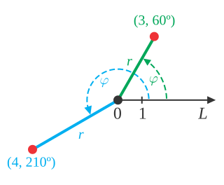
In mathematics, the polar coordinate system is a two-dimensional coordinate system in which each point on a plane is determined by a distance from a reference point and an angle from a reference direction. The reference point is called the pole, and the ray from the pole in the reference direction is the polar axis. The distance from the pole is called the radial coordinate, radial distance or simply radius, and the angle is called the angular coordinate, polar angle, or azimuth. Angles in polar notation are generally expressed in either degrees or radians.

<span class="mw-page-title-main">Spherical coordinate system</span> 3-dimensional coordinate system

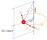
In mathematics, a spherical coordinate system is a coordinate system for three-dimensional space where the position of a point is specified by three numbers: the radial distance of that point from a fixed origin; its polar angle measured from a fixed polar axis or zenith direction; and the azimuthal angle of its orthogonal projection on a reference plane that passes through the origin and is orthogonal to the fixed axis, measured from another fixed reference direction on that plane. When radius is fixed, the two angular coordinates make a coordinate system on the sphere sometimes called spherical polar coordinates.

<span class="mw-page-title-main">Laplace's equation</span> Second-order partial differential equation

In mathematics and physics, Laplace's equation is a second-order partial differential equation named after Pierre-Simon Laplace, who first studied its properties. This is often written as

<span class="mw-page-title-main">Equations of motion</span> Equations that describe the behavior of a physical system

In physics, equations of motion are equations that describe the behavior of a physical system in terms of its motion as a function of time. More specifically, the equations of motion describe the behavior of a physical system as a set of mathematical functions in terms of dynamic variables. These variables are usually spatial coordinates and time, but may include momentum components. The most general choice are generalized coordinates which can be any convenient variables characteristic of the physical system. The functions are defined in a Euclidean space in classical mechanics, but are replaced by curved spaces in relativity. If the dynamics of a system is known, the equations are the solutions for the differential equations describing the motion of the dynamics.

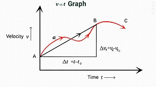
Kinematics is a subfield of physics, developed in classical mechanics, that describes the motion of points, bodies (objects), and systems of bodies without considering the forces that cause them to move. Kinematics, as a field of study, is often referred to as the "geometry of motion" and is occasionally seen as a branch of mathematics. A kinematics problem begins by describing the geometry of the system and declaring the initial conditions of any known values of position, velocity and/or acceleration of points within the system. Then, using arguments from geometry, the position, velocity and acceleration of any unknown parts of the system can be determined. The study of how forces act on bodies falls within kinetics, not kinematics. For further details, see analytical dynamics.

In mathematics, the Laplace operator or Laplacian is a differential operator given by the divergence of the gradient of a scalar function on Euclidean space. It is usually denoted by the symbols , (where is the nabla operator), or . In a Cartesian coordinate system, the Laplacian is given by the sum of second partial derivatives of the function with respect to each independent variable. In other coordinate systems, such as cylindrical and spherical coordinates, the Laplacian also has a useful form. Informally, the Laplacian Δf (p) of a function f at a point p measures by how much the average value of f over small spheres or balls centered at p deviates from f (p).

<span class="mw-page-title-main">Hamiltonian mechanics</span> Formulation of classical mechanics using momenta

Hamiltonian mechanics emerged in 1833 as a reformulation of Lagrangian mechanics. Introduced by Sir William Rowan Hamilton, Hamiltonian mechanics replaces (generalized) velocities used in Lagrangian mechanics with (generalized) momenta. Both theories provide interpretations of classical mechanics and describe the same physical phenomena.

<span class="mw-page-title-main">Spherical harmonics</span> Special mathematical functions defined on the surface of a sphere

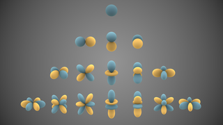
In mathematics and physical science, spherical harmonics are special functions defined on the surface of a sphere. They are often employed in solving partial differential equations in many scientific fields.

<span class="mw-page-title-main">Inverted pendulum</span> Pendulum with center of mass above pivot

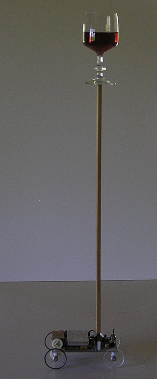
An inverted pendulum is a pendulum that has its center of mass above its pivot point. It is unstable and without additional help will fall over. It can be suspended stably in this inverted position by using a control system to monitor the angle of the pole and move the pivot point horizontally back under the center of mass when it starts to fall over, keeping it balanced. The inverted pendulum is a classic problem in dynamics and control theory and is used as a benchmark for testing control strategies. It is often implemented with the pivot point mounted on a cart that can move horizontally under control of an electronic servo system as shown in the photo; this is called a cart and pole apparatus. Most applications limit the pendulum to 1 degree of freedom by affixing the pole to an axis of rotation. Whereas a normal pendulum is stable when hanging downwards, an inverted pendulum is inherently unstable, and must be actively balanced in order to remain upright; this can be done either by applying a torque at the pivot point, by moving the pivot point horizontally as part of a feedback system, changing the rate of rotation of a mass mounted on the pendulum on an axis parallel to the pivot axis and thereby generating a net torque on the pendulum, or by oscillating the pivot point vertically. A simple demonstration of moving the pivot point in a feedback system is achieved by balancing an upturned broomstick on the end of one's finger.

Linear elasticity is a mathematical model of how solid objects deform and become internally stressed due to prescribed loading conditions. It is a simplification of the more general nonlinear theory of elasticity and a branch of continuum mechanics.

A nonholonomic system in physics and mathematics is a physical system whose state depends on the path taken in order to achieve it. Such a system is described by a set of parameters subject to differential constraints and non-linear constraints, such that when the system evolves along a path in its parameter space but finally returns to the original set of parameter values at the start of the path, the system itself may not have returned to its original state. Nonholonomic mechanics is autonomous division of Newtonian mechanics.

In physics, the Hamilton–Jacobi equation, named after William Rowan Hamilton and Carl Gustav Jacob Jacobi, is an alternative formulation of classical mechanics, equivalent to other formulations such as Newton's laws of motion, Lagrangian mechanics and Hamiltonian mechanics.

In rotordynamics, the rigid rotor is a mechanical model of rotating systems. An arbitrary rigid rotor is a 3-dimensional rigid object, such as a top. To orient such an object in space requires three angles, known as Euler angles. A special rigid rotor is the linear rotor requiring only two angles to describe, for example of a diatomic molecule. More general molecules are 3-dimensional, such as water, ammonia, or methane.

<span class="mw-page-title-main">Routhian mechanics</span> Formulation of classical mechanics

In classical mechanics, Routh's procedure or Routhian mechanics is a hybrid formulation of Lagrangian mechanics and Hamiltonian mechanics developed by Edward John Routh. Correspondingly, the Routhian is the function which replaces both the Lagrangian and Hamiltonian functions. Routhian mechanics is equivalent to Lagrangian mechanics and Hamiltonian mechanics, and introduces no new physics. It offers an alternative way to solve mechanical problems.

In physics, the Green's function for Laplace's equation in three variables is used to describe the response of a particular type of physical system to a point source. In particular, this Green's function arises in systems that can be described by Poisson's equation, a partial differential equation (PDE) of the form

In classical mechanics, holonomic constraints are relations between the position variables that can be expressed in the following form:

In mathematics, vector spherical harmonics (VSH) are an extension of the scalar spherical harmonics for use with vector fields. The components of the VSH are complex-valued functions expressed in the spherical coordinate basis vectors.

In fluid dynamics, the Oseen equations describe the flow of a viscous and incompressible fluid at small Reynolds numbers, as formulated by Carl Wilhelm Oseen in 1910. Oseen flow is an improved description of these flows, as compared to Stokes flow, with the (partial) inclusion of convective acceleration.

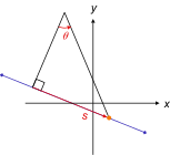
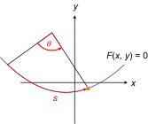
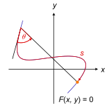
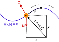
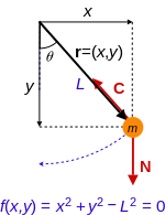
This article describes a particle in planar motion when observed from non-inertial reference frames. The most famous examples of planar motion are related to the motion of two spheres that are gravitationally attracted to one another, and the generalization of this problem to planetary motion. See centrifugal force, two-body problem, orbit and Kepler's laws of planetary motion. These problems fall in the general field of analytical dynamics, determining orbits from the given force laws. This article is focused more on the kinematical issues surrounding planar motion, that is, the determination of the forces necessary to result in a certain trajectory given the particle trajectory.

<span class="mw-page-title-main">Lagrangian mechanics</span> Formulation of classical mechanics

In physics, Lagrangian mechanics is a formulation of classical mechanics founded on the stationary-action principle. It was introduced by the Italian-French mathematician and astronomer Joseph-Louis Lagrange in his 1788 work, Mécanique analytique.

References

  1. Ginsberg 2008, p. 397,  §7.2.1 Selection of generalized coordinates
  2. Farid M. L. Amirouche (2006). "§2.4: Generalized coordinates". Fundamentals of multibody dynamics: theory and applications. Springer. p. 46. ISBN   0-8176-4236-6.
  3. Florian Scheck (2010). "§5.1 Manifolds of generalized coordinates". Mechanics: From Newton's Laws to Deterministic Chaos (5th ed.). Springer. p. 286. ISBN   978-3-642-05369-6.
  4. Goldstein, Poole & Safko 2002 , p. 12
  5. 1 2 Kibble & Berkshire 2004 , p. 232
  6. Torby 1984 , p. 260
  7. Goldstein, Poole & Safko 2002 , p. 13
  8. Hand & Finch 1998 , p. 15
  9. Torby 1984 , p. 269
  10. Goldstein, Poole & Safko 2002 , p. 25
  11. Landau & Lifshitz 1976 , p. 8
  12. Greenwood, Donald T. (1987). Principles of Dynamics (2nd ed.). Prentice Hall. ISBN   0-13-709981-9.
  13. Richard Fitzpatrick, Newtonian Dynamics.
  14. Eric W. Weisstein, Double Pendulum, scienceworld.wolfram.com. 2007
  15. Torby 1984
  16. T. R. Kane and D. A. Levinson, Dynamics: theory and applications, McGraw-Hill, New York, 1985

Bibliography of cited references