Manifold regularization

Last updated
Manifold regularization can classify data when labeled data (black and white circles) are sparse, by taking advantage of unlabeled data (gray circles). Without many labeled data points, supervised learning algorithms can only learn very simple decision boundaries (top panel). Manifold learning can draw a decision boundary between the natural classes of the unlabeled data, under the assumption that close-together points probably belong to the same class, and so the decision boundary should avoid areas with many unlabeled points. This is one version of semi-supervised learning. Example of unlabeled data in semisupervised learning.png
Manifold regularization can classify data when labeled data (black and white circles) are sparse, by taking advantage of unlabeled data (gray circles). Without many labeled data points, supervised learning algorithms can only learn very simple decision boundaries (top panel). Manifold learning can draw a decision boundary between the natural classes of the unlabeled data, under the assumption that close-together points probably belong to the same class, and so the decision boundary should avoid areas with many unlabeled points. This is one version of semi-supervised learning.

In machine learning, Manifold regularization is a technique for using the shape of a dataset to constrain the functions that should be learned on that dataset. In many machine learning problems, the data to be learned do not cover the entire input space. For example, a facial recognition system may not need to classify any possible image, but only the subset of images that contain faces. The technique of manifold learning assumes that the relevant subset of data comes from a manifold, a mathematical structure with useful properties. The technique also assumes that the function to be learned is smooth: data with different labels are not likely to be close together, and so the labeling function should not change quickly in areas where there are likely to be many data points. Because of this assumption, a manifold regularization algorithm can use unlabeled data to inform where the learned function is allowed to change quickly and where it is not, using an extension of the technique of Tikhonov regularization. Manifold regularization algorithms can extend supervised learning algorithms in semi-supervised learning and transductive learning settings, where unlabeled data are available. The technique has been used for applications including medical imaging, geographical imaging, and object recognition.

Contents

Manifold regularizer

Motivation

Manifold regularization is a type of regularization, a family of techniques that reduces overfitting and ensures that a problem is well-posed by penalizing complex solutions. In particular, manifold regularization extends the technique of Tikhonov regularization as applied to Reproducing kernel Hilbert spaces (RKHSs). Under standard Tikhonov regularization on RKHSs, a learning algorithm attempts to learn a function from among a hypothesis space of functions . The hypothesis space is an RKHS, meaning that it is associated with a kernel , and so every candidate function has a norm , which represents the complexity of the candidate function in the hypothesis space. When the algorithm considers a candidate function, it takes its norm into account in order to penalize complex functions.

Formally, given a set of labeled training data with and a loss function , a learning algorithm using Tikhonov regularization will attempt to solve the expression

where is a hyperparameter that controls how much the algorithm will prefer simpler functions over functions that fit the data better.

A two-dimensional manifold embedded in three-dimensional space (left). Manifold regularization attempts to learn a function that is smooth on the unrolled manifold (right). Swissroll manifold unrolled.png
A two-dimensional manifold embedded in three-dimensional space (left). Manifold regularization attempts to learn a function that is smooth on the unrolled manifold (right).

Manifold regularization adds a second regularization term, the intrinsic regularizer, to the ambient regularizer used in standard Tikhonov regularization. Under the manifold assumption in machine learning, the data in question do not come from the entire input space , but instead from a nonlinear manifold . The geometry of this manifold, the intrinsic space, is used to determine the regularization norm. [1]

Laplacian norm

There are many possible choices for the intrinsic regularizer . Many natural choices involve the gradient on the manifold , which can provide a measure of how smooth a target function is. A smooth function should change slowly where the input data are dense; that is, the gradient should be small where the marginal probability density, the probability density of a randomly drawn data point appearing at , is large. This gives one appropriate choice for the intrinsic regularizer:

In practice, this norm cannot be computed directly because the marginal distribution is unknown, but it can be estimated from the provided data.

Graph-based approach of the Laplacian norm

When the distances between input points are interpreted as a graph, then the Laplacian matrix of the graph can help to estimate the marginal distribution. Suppose that the input data include labeled examples (pairs of an input and a label ) and unlabeled examples (inputs without associated labels). Define to be a matrix of edge weights for a graph, where is a distance measure between the data points and . Define to be a diagonal matrix with and to be the Laplacian matrix . Then, as the number of data points increases, converges to the Laplace–Beltrami operator , which is the divergence of the gradient . [2] [3] Then, if is a vector of the values of at the data, , the intrinsic norm can be estimated:

As the number of data points increases, this empirical definition of converges to the definition when is known. [1]

Solving the regularization problem with graph-based approach

Using the weights and for the ambient and intrinsic regularizers, the final expression to be solved becomes:

As with other kernel methods, may be an infinite-dimensional space, so if the regularization expression cannot be solved explicitly, it is impossible to search the entire space for a solution. Instead, a representer theorem shows that under certain conditions on the choice of the norm , the optimal solution must be a linear combination of the kernel centered at each of the input points: for some weights ,

Using this result, it is possible to search for the optimal solution by searching the finite-dimensional space defined by the possible choices of . [1]

Functional approach of the Laplacian norm

The idea beyond graph-Laplacian is to use neighbors to estimate Laplacian. This method is akin local averaging methods, that are known to scale poorly in high-dimensional problem. Indeed, graph Laplacian is known to suffer from the curse of dimensionality. [2] Luckily, it is possible to leverage expected smoothness of the function to estimate thanks to more advanced functional analysis. This method consists in estimating the Laplacian operator thanks to derivatives of the kernel reading where denotes the partial derivatives according to the j-th coordinate of the first variable. [4] This second approach of the Laplacian norm is to put in relation with meshfree methods, that contrast with the finite difference method in PDE.

Applications

Manifold regularization can extend a variety of algorithms that can be expressed using Tikhonov regularization, by choosing an appropriate loss function and hypothesis space . Two commonly used examples are the families of support vector machines and regularized least squares algorithms. (Regularized least squares includes the ridge regression algorithm; the related algorithms of LASSO and elastic net regularization can be expressed as support vector machines. [5] [6] ) The extended versions of these algorithms are called Laplacian Regularized Least Squares (abbreviated LapRLS) and Laplacian Support Vector Machines (LapSVM), respectively. [1]

Laplacian Regularized Least Squares (LapRLS)

Regularized least squares (RLS) is a family of regression algorithms: algorithms that predict a value for its inputs , with the goal that the predicted values should be close to the true labels for the data. In particular, RLS is designed to minimize the mean squared error between the predicted values and the true labels, subject to regularization. Ridge regression is one form of RLS; in general, RLS is the same as ridge regression combined with the kernel method.[ citation needed ] The problem statement for RLS results from choosing the loss function in Tikhonov regularization to be the mean squared error:

Thanks to the representer theorem, the solution can be written as a weighted sum of the kernel evaluated at the data points:

and solving for gives:

where is defined to be the kernel matrix, with , and is the vector of data labels.

Adding a Laplacian term for manifold regularization gives the Laplacian RLS statement:

The representer theorem for manifold regularization again gives

and this yields an expression for the vector . Letting be the kernel matrix as above, be the vector of data labels, and be the block matrix :

with a solution of

[1]

LapRLS has been applied to problems including sensor networks, [7] medical imaging, [8] [9] object detection, [10] spectroscopy, [11] document classification, [12] drug-protein interactions, [13] and compressing images and videos. [14]

Laplacian Support Vector Machines (LapSVM)

Support vector machines (SVMs) are a family of algorithms often used for classifying data into two or more groups, or classes. Intuitively, an SVM draws a boundary between classes so that the closest labeled examples to the boundary are as far away as possible. This can be directly expressed as a linear program, but it is also equivalent to Tikhonov regularization with the hinge loss function, :

[15] [16]

Adding the intrinsic regularization term to this expression gives the LapSVM problem statement:

Again, the representer theorem allows the solution to be expressed in terms of the kernel evaluated at the data points:

can be found by writing the problem as a linear program and solving the dual problem. Again letting be the kernel matrix and be the block matrix , the solution can be shown to be

where is the solution to the dual problem

and is defined by

[1]

LapSVM has been applied to problems including geographical imaging, [17] [18] [19] medical imaging, [20] [21] [22] face recognition, [23] machine maintenance, [24] and brain–computer interfaces. [25]

Limitations

See also

Related Research Articles

In machine learning, support vector machines are supervised max-margin models with associated learning algorithms that analyze data for classification and regression analysis. Developed at AT&T Bell Laboratories by Vladimir Vapnik with colleagues SVMs are one of the most studied models, being based on statistical learning frameworks or VC theory proposed by Vapnik and Chervonenkis (1974).

<span class="mw-page-title-main">Gamma distribution</span> Probability distribution

In probability theory and statistics, the gamma distribution is a two-parameter family of continuous probability distributions. The exponential distribution, Erlang distribution, and chi-squared distribution are special cases of the gamma distribution. There are two equivalent parameterizations in common use:

  1. With a shape parameter k and a scale parameter θ
  2. With a shape parameter and an inverse scale parameter , called a rate parameter.

In mathematics, the Riemann–Liouville integral associates with a real function another function Iαf of the same kind for each value of the parameter α > 0. The integral is a manner of generalization of the repeated antiderivative of f in the sense that for positive integer values of α, Iαf is an iterated antiderivative of f of order α. The Riemann–Liouville integral is named for Bernhard Riemann and Joseph Liouville, the latter of whom was the first to consider the possibility of fractional calculus in 1832. The operator agrees with the Euler transform, after Leonhard Euler, when applied to analytic functions. It was generalized to arbitrary dimensions by Marcel Riesz, who introduced the Riesz potential.

Multi-task learning (MTL) is a subfield of machine learning in which multiple learning tasks are solved at the same time, while exploiting commonalities and differences across tasks. This can result in improved learning efficiency and prediction accuracy for the task-specific models, when compared to training the models separately. Early versions of MTL were called "hints".

In rotordynamics, the rigid rotor is a mechanical model of rotating systems. An arbitrary rigid rotor is a 3-dimensional rigid object, such as a top. To orient such an object in space requires three angles, known as Euler angles. A special rigid rotor is the linear rotor requiring only two angles to describe, for example of a diatomic molecule. More general molecules are 3-dimensional, such as water, ammonia, or methane.

<span class="mw-page-title-main">Regularization (mathematics)</span> Technique to make a model more generalizable and transferable

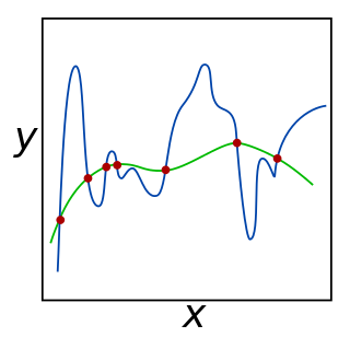
In mathematics, statistics, finance, computer science, particularly in machine learning and inverse problems, regularization is a process that changes the result answer to be "simpler". It is often used to obtain results for ill-posed problems or to prevent overfitting.

The Wigner D-matrix is a unitary matrix in an irreducible representation of the groups SU(2) and SO(3). It was introduced in 1927 by Eugene Wigner, and plays a fundamental role in the quantum mechanical theory of angular momentum. The complex conjugate of the D-matrix is an eigenfunction of the Hamiltonian of spherical and symmetric rigid rotors. The letter D stands for Darstellung, which means "representation" in German.

Linear Programming Boosting (LPBoost) is a supervised classifier from the boosting family of classifiers. LPBoost maximizes a margin between training samples of different classes and hence also belongs to the class of margin-maximizing supervised classification algorithms. Consider a classification function

Gradient boosting is a machine learning technique based on boosting in a functional space, where the target is pseudo-residuals rather than the typical residuals used in traditional boosting. It gives a prediction model in the form of an ensemble of weak prediction models, i.e., models that make very few assumptions about the data, which are typically simple decision trees. When a decision tree is the weak learner, the resulting algorithm is called gradient-boosted trees; it usually outperforms random forest. A gradient-boosted trees model is built in a stage-wise fashion as in other boosting methods, but it generalizes the other methods by allowing optimization of an arbitrary differentiable loss function.

In mathematics, the Kodaira–Spencer map, introduced by Kunihiko Kodaira and Donald C. Spencer, is a map associated to a deformation of a scheme or complex manifold X, taking a tangent space of a point of the deformation space to the first cohomology group of the sheaf of vector fields on X.

<span class="mw-page-title-main">Relativistic angular momentum</span> Angular momentum in special and general relativity

In physics, relativistic angular momentum refers to the mathematical formalisms and physical concepts that define angular momentum in special relativity (SR) and general relativity (GR). The relativistic quantity is subtly different from the three-dimensional quantity in classical mechanics.

Proximal gradientmethods for learning is an area of research in optimization and statistical learning theory which studies algorithms for a general class of convex regularization problems where the regularization penalty may not be differentiable. One such example is regularization of the form

In machine learning, the kernel embedding of distributions comprises a class of nonparametric methods in which a probability distribution is represented as an element of a reproducing kernel Hilbert space (RKHS). A generalization of the individual data-point feature mapping done in classical kernel methods, the embedding of distributions into infinite-dimensional feature spaces can preserve all of the statistical features of arbitrary distributions, while allowing one to compare and manipulate distributions using Hilbert space operations such as inner products, distances, projections, linear transformations, and spectral analysis. This learning framework is very general and can be applied to distributions over any space on which a sensible kernel function may be defined. For example, various kernels have been proposed for learning from data which are: vectors in , discrete classes/categories, strings, graphs/networks, images, time series, manifolds, dynamical systems, and other structured objects. The theory behind kernel embeddings of distributions has been primarily developed by Alex Smola, Le Song , Arthur Gretton, and Bernhard Schölkopf. A review of recent works on kernel embedding of distributions can be found in.

<span class="mw-page-title-main">Causal fermion systems</span> Candidate unified theory of physics

The theory of causal fermion systems is an approach to describe fundamental physics. It provides a unification of the weak, the strong and the electromagnetic forces with gravity at the level of classical field theory. Moreover, it gives quantum mechanics as a limiting case and has revealed close connections to quantum field theory. Therefore, it is a candidate for a unified physical theory. Instead of introducing physical objects on a preexisting spacetime manifold, the general concept is to derive spacetime as well as all the objects therein as secondary objects from the structures of an underlying causal fermion system. This concept also makes it possible to generalize notions of differential geometry to the non-smooth setting. In particular, one can describe situations when spacetime no longer has a manifold structure on the microscopic scale. As a result, the theory of causal fermion systems is a proposal for quantum geometry and an approach to quantum gravity.

Multiple kernel learning refers to a set of machine learning methods that use a predefined set of kernels and learn an optimal linear or non-linear combination of kernels as part of the algorithm. Reasons to use multiple kernel learning include a) the ability to select for an optimal kernel and parameters from a larger set of kernels, reducing bias due to kernel selection while allowing for more automated machine learning methods, and b) combining data from different sources that have different notions of similarity and thus require different kernels. Instead of creating a new kernel, multiple kernel algorithms can be used to combine kernels already established for each individual data source.

Regularized least squares (RLS) is a family of methods for solving the least-squares problem while using regularization to further constrain the resulting solution.

In statistical learning theory, a learnable function class is a set of functions for which an algorithm can be devised to asymptotically minimize the expected risk, uniformly over all probability distributions. The concept of learnable classes are closely related to regularization in machine learning, and provides large sample justifications for certain learning algorithms.

The convolutional sparse coding paradigm is an extension of the global sparse coding model, in which a redundant dictionary is modeled as a concatenation of circulant matrices. While the global sparsity constraint describes signal as a linear combination of a few atoms in the redundant dictionary , usually expressed as for a sparse vector , the alternative dictionary structure adopted by the convolutional sparse coding model allows the sparsity prior to be applied locally instead of globally: independent patches of are generated by "local" dictionaries operating over stripes of .

Weak supervision is a paradigm in machine learning, the relevance and notability of which increased with the advent of large language models due to large amount of data required to train them. It is characterized by using a combination of a small amount of human-labeled data, followed by a large amount of unlabeled data. In other words, the desired output values are provided only for a subset of the training data. The remaining data is unlabeled or imprecisely labeled. Intuitively, it can be seen as an exam and labeled data as sample problems that the teacher solves for the class as an aid in solving another set of problems. In the transductive setting, these unsolved problems act as exam questions. In the inductive setting, they become practice problems of the sort that will make up the exam. Technically, it could be viewed as performing clustering and then labeling the clusters with the labeled data, pushing the decision boundary away from high-density regions, or learning an underlying one-dimensional manifold where the data reside.

In complex geometry, the lemma is a mathematical lemma about the de Rham cohomology class of a complex differential form. The -lemma is a result of Hodge theory and the Kähler identities on a compact Kähler manifold. Sometimes it is also known as the -lemma, due to the use of a related operator , with the relation between the two operators being and so .

References

  1. 1 2 3 4 5 6 Belkin, Mikhail; Niyogi, Partha; Sindhwani, Vikas (2006). "Manifold regularization: A geometric framework for learning from labeled and unlabeled examples". The Journal of Machine Learning Research. 7: 2399–2434. Retrieved 2015-12-02.
  2. 1 2 Hein, Matthias; Audibert, Jean-Yves; Von Luxburg, Ulrike (2005). "From graphs to manifolds–weak and strong pointwise consistency of graph laplacians". Learning theory. Lecture Notes in Computer Science. Vol. 3559. Springer. pp. 470–485. CiteSeerX   10.1.1.103.82 . doi:10.1007/11503415_32. ISBN   978-3-540-26556-6.
  3. Belkin, Mikhail; Niyogi, Partha (2005). "Towards a theoretical foundation for Laplacian-based manifold methods". Learning theory. Lecture Notes in Computer Science. Vol. 3559. Springer. pp. 486–500. CiteSeerX   10.1.1.127.795 . doi:10.1007/11503415_33. ISBN   978-3-540-26556-6.
  4. Cabannes, Vivien; Pillaud-Vivien, Loucas; Bach, Francis; Rudi, Alessandro (2021). "Overcoming the curse of dimensionality with Laplacian regularization in semi-supervised learning". arXiv: 2009.04324 [stat.ML].
  5. Jaggi, Martin (2014). Suykens, Johan; Signoretto, Marco; Argyriou, Andreas (eds.). An Equivalence between the Lasso and Support Vector Machines. Chapman and Hall/CRC.
  6. Zhou, Quan; Chen, Wenlin; Song, Shiji; Gardner, Jacob; Weinberger, Kilian; Chen, Yixin. A Reduction of the Elastic Net to Support Vector Machines with an Application to GPU Computing. Association for the Advancement of Artificial Intelligence.
  7. Pan, Jeffrey Junfeng; Yang, Qiang; Chang, Hong; Yeung, Dit-Yan (2006). "A manifold regularization approach to calibration reduction for sensor-network based tracking" (PDF). Proceedings of the national conference on artificial intelligence. Vol. 21. Menlo Park, CA; Cambridge, MA; London; AAAI Press; MIT Press; 1999. p. 988. Retrieved 2015-12-02.
  8. Zhang, Daoqiang; Shen, Dinggang (2011). "Semi-supervised multimodal classification of Alzheimer's disease". Biomedical Imaging: From Nano to Macro, 2011 IEEE International Symposium on. IEEE. pp. 1628–1631. doi:10.1109/ISBI.2011.5872715.
  9. Park, Sang Hyun; Gao, Yaozong; Shi, Yinghuan; Shen, Dinggang (2014). "Interactive Prostate Segmentation Based on Adaptive Feature Selection and Manifold Regularization". Machine Learning in Medical Imaging. Lecture Notes in Computer Science. Vol. 8679. Springer. pp. 264–271. doi:10.1007/978-3-319-10581-9_33. ISBN   978-3-319-10580-2.
  10. Pillai, Sudeep. "Semi-supervised Object Detector Learning from Minimal Labels" (PDF). Retrieved 2015-12-15.{{cite journal}}: Cite journal requires |journal= (help)
  11. Wan, Songjing; Wu, Di; Liu, Kangsheng (2012). "Semi-Supervised Machine Learning Algorithm in Near Infrared Spectral Calibration: A Case Study on Diesel Fuels". Advanced Science Letters. 11 (1): 416–419. doi:10.1166/asl.2012.3044.
  12. Wang, Ziqiang; Sun, Xia; Zhang, Lijie; Qian, Xu (2013). "Document Classification based on Optimal Laprls". Journal of Software. 8 (4): 1011–1018. doi:10.4304/jsw.8.4.1011-1018.
  13. Xia, Zheng; Wu, Ling-Yun; Zhou, Xiaobo; Wong, Stephen TC (2010). "Semi-supervised drug-protein interaction prediction from heterogeneous biological spaces". BMC Systems Biology. 4 (Suppl 2): –6. CiteSeerX   10.1.1.349.7173 . doi: 10.1186/1752-0509-4-S2-S6 . PMC   2982693 . PMID   20840733.
  14. Cheng, Li; Vishwanathan, S. V. N. (2007). "Learning to compress images and videos". Proceedings of the 24th international conference on Machine learning. ACM. pp. 161–168. Retrieved 2015-12-16.
  15. Lin, Yi; Wahba, Grace; Zhang, Hao; Lee, Yoonkyung (2002). "Statistical properties and adaptive tuning of support vector machines". Machine Learning. 48 (1–3): 115–136. doi: 10.1023/A:1013951620650 .
  16. Wahba, Grace; others (1999). "Support vector machines, reproducing kernel Hilbert spaces and the randomized GACV". Advances in Kernel Methods-Support Vector Learning. 6: 69–87. CiteSeerX   10.1.1.53.2114 .
  17. Kim, Wonkook; Crawford, Melba M. (2010). "Adaptive classification for hyperspectral image data using manifold regularization kernel machines". IEEE Transactions on Geoscience and Remote Sensing. 48 (11): 4110–4121. doi:10.1109/TGRS.2010.2076287. S2CID   29580629.
  18. Camps-Valls, Gustavo; Tuia, Devis; Bruzzone, Lorenzo; Atli Benediktsson, Jon (2014). "Advances in hyperspectral image classification: Earth monitoring with statistical learning methods". IEEE Signal Processing Magazine. 31 (1): 45–54. arXiv: 1310.5107 . Bibcode:2014ISPM...31...45C. doi:10.1109/msp.2013.2279179. S2CID   11945705.
  19. Gómez-Chova, Luis; Camps-Valls, Gustavo; Muñoz-Marí, Jordi; Calpe, Javier (2007). "Semi-supervised cloud screening with Laplacian SVM". Geoscience and Remote Sensing Symposium, 2007. IGARSS 2007. IEEE International. IEEE. pp. 1521–1524. doi:10.1109/IGARSS.2007.4423098.
  20. Cheng, Bo; Zhang, Daoqiang; Shen, Dinggang (2012). "Domain transfer learning for MCI conversion prediction". Medical Image Computing and Computer-Assisted Intervention–MICCAI 2012. Lecture Notes in Computer Science. Vol. 7510. Springer. pp. 82–90. doi:10.1007/978-3-642-33415-3_11. ISBN   978-3-642-33414-6. PMC   3761352 . PMID   23285538.
  21. Jamieson, Andrew R.; Giger, Maryellen L.; Drukker, Karen; Pesce, Lorenzo L. (2010). "Enhancement of breast CADx with unlabeled dataa)". Medical Physics. 37 (8): 4155–4172. Bibcode:2010MedPh..37.4155J. doi:10.1118/1.3455704. PMC   2921421 . PMID   20879576.
  22. Wu, Jiang; Diao, Yuan-Bo; Li, Meng-Long; Fang, Ya-Ping; Ma, Dai-Chuan (2009). "A semi-supervised learning based method: Laplacian support vector machine used in diabetes disease diagnosis". Interdisciplinary Sciences: Computational Life Sciences. 1 (2): 151–155. doi:10.1007/s12539-009-0016-2. PMID   20640829. S2CID   21860700.
  23. Wang, Ziqiang; Zhou, Zhiqiang; Sun, Xia; Qian, Xu; Sun, Lijun (2012). "Enhanced LapSVM Algorithm for Face Recognition". International Journal of Advancements in Computing Technology. 4 (17). Retrieved 2015-12-16.
  24. Zhao, Xiukuan; Li, Min; Xu, Jinwu; Song, Gangbing (2011). "An effective procedure exploiting unlabeled data to build monitoring system". Expert Systems with Applications. 38 (8): 10199–10204. doi:10.1016/j.eswa.2011.02.078.
  25. Zhong, Ji-Ying; Lei, Xu; Yao, D. (2009). "Semi-supervised learning based on manifold in BCI" (PDF). Journal of Electronics Science and Technology of China. 7 (1): 22–26. Retrieved 2015-12-16.
  26. Zhu, Xiaojin (2005). "Semi-supervised learning literature survey". CiteSeerX   10.1.1.99.9681 .{{cite journal}}: Cite journal requires |journal= (help)
  27. Sindhwani, Vikas; Rosenberg, David S. (2008). "An RKHS for multi-view learning and manifold co-regularization". Proceedings of the 25th international conference on Machine learning. ACM. pp. 976–983. Retrieved 2015-12-02.
  28. Goldberg, Andrew; Li, Ming; Zhu, Xiaojin (2008). "Online Manifold Regularization: A New Learning Setting and Empirical Study". Machine Learning and Knowledge Discovery in Databases. Lecture Notes in Computer Science. Vol. 5211. pp. 393–407. doi:10.1007/978-3-540-87479-9_44. ISBN   978-3-540-87478-2.

Software