Projectile motion

Last updated
Parabolic water motion trajectory ParabolicWaterTrajectory.jpg
Parabolic water motion trajectory
Components of initial velocity of parabolic throwing Ferde hajitas2.svg
Components of initial velocity of parabolic throwing
Ballistic trajectories are parabolic if gravity is homogeneous and elliptic if it is round. Ballistic trajectories.svg
Ballistic trajectories are parabolic if gravity is homogeneous and elliptic if it is round.

Projectile motion is a form of motion experienced by an object or particle (a projectile) that is projected in a gravitational field, such as from Earth's surface, and moves along a curved path under the action of gravity only. In the particular case of projectile motion on Earth, most calculations assume the effects of air resistance are passive and negligible. The curved path of objects in projectile motion was shown by Galileo to be a parabola, but may also be a straight line in the special case when it is thrown directly upward or downward. The study of such motions is called ballistics, and such a trajectory is a ballistic trajectory. The only force of mathematical significance that is actively exerted on the object is gravity, which acts downward, thus imparting to the object a downward acceleration towards the Earth’s center of mass. Because of the object's inertia, no external force is needed to maintain the horizontal velocity component of the object's motion. Taking other forces into account, such as aerodynamic drag or internal propulsion (such as in a rocket), requires additional analysis. A ballistic missile is a missile only guided during the relatively brief initial powered phase of flight, and whose remaining course is governed by the laws of classical mechanics.

Contents

Ballistics (from Ancient Greek βάλλειν bállein 'to throw') is the science of dynamics that deals with the flight, behavior and effects of projectiles, especially bullets, unguided bombs, rockets, or the like; the science or art of designing and accelerating projectiles so as to achieve a desired performance.

Trajectories of a projectile with air drag and varying initial velocities Mplwp ballistic trajectories velocities.svg
Trajectories of a projectile with air drag and varying initial velocities

The elementary equation of ballistics neglect nearly every factor except for initial velocity and an assumed constant gravitational acceleration. Practical solutions of a ballistics problem often require considerations of air resistance, cross winds, target motion, varying acceleration due to gravity, and in such problems as launching a rocket from one point on the Earth to another, the rotation of the Earth. Detailed mathematical solutions of practical problems typically do not have closed-form solutions, and therefore require numerical methods to address.

Kinematic quantities

In projectile motion, the horizontal motion and the vertical motion are independent of each other; that is, neither motion affects the other. This is the principle of compound motion established by Galileo in 1638, [1] and used by him to prove the parabolic form of projectile motion. [2]

The horizontal and vertical components of a projectile's velocity are independent of each other. Compound Motion.gif
The horizontal and vertical components of a projectile's velocity are independent of each other.

A ballistic trajectory is a parabola with homogeneous acceleration, such as in a space ship with constant acceleration in absence of other forces. On Earth the acceleration changes magnitude with altitude and direction with latitude/longitude. This causes an elliptic trajectory, which is very close to a parabola on a small scale. However, if an object was thrown and the Earth was suddenly replaced with a black hole of equal mass, it would become obvious that the ballistic trajectory is part of an elliptic orbit around that black hole, and not a parabola that extends to infinity. At higher speeds the trajectory can also be circular, parabolic or hyperbolic (unless distorted by other objects like the Moon or the Sun). In this article a homogeneous acceleration is assumed.

Acceleration

Since there is acceleration only in the vertical direction, the velocity in the horizontal direction is constant, being equal to . The vertical motion of the projectile is the motion of a particle during its free fall. Here the acceleration is constant, being equal to g. [note 1] The components of the acceleration are:

,
.*


*The y acceleration can also be referred to as the force of the earth on the object(s) of interest.

Velocity

Let the projectile be launched with an initial velocity , which can be expressed as the sum of horizontal and vertical components as follows:

.

The components and can be found if the initial launch angle, , is known:

,

The horizontal component of the velocity of the object remains unchanged throughout the motion. The vertical component of the velocity changes linearly, [note 2] because the acceleration due to gravity is constant. The accelerations in the x and y directions can be integrated to solve for the components of velocity at any time t, as follows:

,
.

The magnitude of the velocity (under the Pythagorean theorem, also known as the triangle law):

.

Displacement

Displacement and coordinates of parabolic throwing Ferde hajitas3.svg
Displacement and coordinates of parabolic throwing

At any time , the projectile's horizontal and vertical displacement are:

,
.

The magnitude of the displacement is:

.

Consider the equations,

[3] .

If t is eliminated between these two equations the following equation is obtained:

Here R is the Range of a projectile.

Since g, θ, and v0 are constants, the above equation is of the form

,

in which a and b are constants. This is the equation of a parabola, so the path is parabolic. The axis of the parabola is vertical.

If the projectile's position (x,y) and launch angle (θ or α) are known, the initial velocity can be found solving for v0 in the aforementioned parabolic equation:

.

Displacement in polar coordinates

The parabolic trajectory of a projectile can also be expressed in polar coordinates instead of Cartesian coordinates. In this case, the position has the general formula

.

In this equation, the origin is the midpoint of the horizontal range of the projectile, and if the ground is flat, the parabolic arc is plotted in the range . This expression can be obtained by transforming the Cartesian equation as stated above by and .

Properties of the trajectory

Time of flight or total time of the whole journey

The total time t for which the projectile remains in the air is called the time of flight.

After the flight, the projectile returns to the horizontal axis (x-axis), so .

Note that we have neglected air resistance on the projectile.

If the starting point is at height y0 with respect to the point of impact, the time of flight is:

As above, this expression can be reduced to

if θ is 45° and y0 is 0.

Time of flight to the target's position

As shown above in the Displacement section, the horizontal and vertical velocity of a projectile are independent of each other.

Because of this, we can find the time to reach a target using the displacement formula for the horizontal velocity:


This equation will give the total time t the projectile must travel for to reach the target's horizontal displacement, neglecting air resistance.

Maximum height of projectile

Maximum height of projectile Ferde hajitas4.svg
Maximum height of projectile

The greatest height that the object will reach is known as the peak of the object's motion. The increase in height will last until , that is,

.

Time to reach the maximum height(h):

.

For the vertical displacement of the maximum height of the projectile:

The maximum reachable height is obtained for θ=90°:

If the projectile's position (x,y) and launch angle (θ) are known, the maximum height can be found by solving for h in the following equation:

Angle of elevation (φ) at the maximum height is given by:

Relation between horizontal range and maximum height

The relation between the range d on the horizontal plane and the maximum height h reached at is:

Proof

×

.

If

Maximum distance of projectile

The maximum distance of projectile Ferde hajitas5.svg
The maximum distance of projectile

The range and the maximum height of the projectile does not depend upon its mass. Hence range and maximum height are equal for all bodies that are thrown with the same velocity and direction. The horizontal range d of the projectile is the horizontal distance it has traveled when it returns to its initial height ().

.

Time to reach ground:

.

From the horizontal displacement the maximum distance of projectile:

,

so [note 3]

.

Note that d has its maximum value when

,

which necessarily corresponds to

,

or

.
Trajectories of projectiles launched at different elevation angles but the same speed of 10 m/s in a vacuum and uniform downward gravity field of 10 m/s . Points are at 0.05 s intervals and length of their tails is linearly proportional to their speed. t = time from launch, T = time of flight, R = range and H = highest point of trajectory (indicated with arrows). Ideal projectile motion for different angles.svg
Trajectories of projectiles launched at different elevation angles but the same speed of 10 m/s in a vacuum and uniform downward gravity field of 10 m/s . Points are at 0.05 s intervals and length of their tails is linearly proportional to their speed. t = time from launch, T = time of flight, R = range and H = highest point of trajectory (indicated with arrows).

The total horizontal distance (d) traveled.

When the surface is flat (initial height of the object is zero), the distance traveled: [4]

Thus the maximum distance is obtained if θ is 45 degrees. This distance is:

Application of the work energy theorem

According to the work-energy theorem the vertical component of velocity is:

.


These formulae ignore aerodynamic drag and also assume that the landing area is at uniform height 0.

Angle of reach

The "angle of reach" is the angle (θ) at which a projectile must be launched in order to go a distance d, given the initial velocity v.

There are two solutions:

(shallow trajectory)

and because ,

(steep trajectory)

Angle θ required to hit coordinate (x, y)

Vacuum trajectory of a projectile for different launch angles. Launch speed is the same for all angles, 50 m/s if "g" is 10 m/s . Trajectory for changing launch angle.gif
Vacuum trajectory of a projectile for different launch angles. Launch speed is the same for all angles, 50 m/s if "g" is 10 m/s .

To hit a target at range x and altitude y when fired from (0,0) and with initial speed v the required angle(s) of launch θ are:

The two roots of the equation correspond to the two possible launch angles, so long as they aren't imaginary, in which case the initial speed is not great enough to reach the point (x,y) selected. This formula allows one to find the angle of launch needed without the restriction of .

One can also ask what launch angle allows the lowest possible launch velocity. This occurs when the two solutions above are equal, implying that the quantity under the square root sign is zero. This requires solving a quadratic equation for , and we find

This gives

If we denote the angle whose tangent is y/x by α, then

This implies

In other words, the launch should be at the angle halfway between the target and Zenith (vector opposite to Gravity)

Total Path Length of the Trajectory

The length of the parabolic arc traced by a projectile L, given that the height of launch and landing is the same and that there is no air resistance, is given by the formula:

where is the initial velocity, is the launch angle and is the acceleration due to gravity as a positive value. The expression can be obtained by evaluating the arc length integral for the height-distance parabola between the bounds initial and final displacements (i.e. between 0 and the horizontal range of the projectile) such that:

If the time of flight is t,

Trajectory of a projectile with air resistance

Trajectories of a mass thrown at an angle of 70deg:

.mw-parser-output .legend{page-break-inside:avoid;break-inside:avoid-column}.mw-parser-output .legend-color{display:inline-block;min-width:1.25em;height:1.25em;line-height:1.25;margin:1px 0;text-align:center;border:1px solid black;background-color:transparent;color:black}.mw-parser-output .legend-text{}
without drag

with Stokes' drag

with Newtonian drag Inclinedthrow2.gif
Trajectories of a mass thrown at an angle of 70°:
  without drag
  with Stokes' drag
  with Newtonian drag

Air resistance creates a force that (for symmetric projectiles) is always directed against the direction of motion in the surrounding medium and has a magnitude that depends on the absolute speed: . The speed-dependence of the friction force is linear () at very low speeds (Stokes drag) and quadratic () at larger speeds (Newton drag). [5] The transition between these behaviours is determined by the Reynolds number, which depends on speed, object size and kinematic viscosity of the medium. For Reynolds numbers below about 1000, the dependence is linear, above it becomes quadratic. In air, which has a kinematic viscosity around , this means that the drag force becomes quadratic in v when the product of speed and diameter is more than about , which is typically the case for projectiles.

Free body diagram of a body on which only gravity and air resistance acts Free body diagram gravity air resistance.svg
Free body diagram of a body on which only gravity and air resistance acts

The free body diagram on the right is for a projectile that experiences air resistance and the effects of gravity. Here, air resistance is assumed to be in the direction opposite of the projectile's velocity:

Trajectory of a projectile with Stokes drag

Stokes drag, where , only applies at very low speed in air, and is thus not the typical case for projectiles. However, the linear dependence of on causes a very simple differential equation of motion

in which the two cartesian components become completely independent, and thus easier to solve. [6] Here, , and will be used to denote the initial velocity, the velocity along the direction of x and the velocity along the direction of y, respectively. The mass of the projectile will be denoted by m, and . For the derivation only the case where is considered. Again, the projectile is fired from the origin (0,0).

Derivation of horizontal position

The relationships that represent the motion of the particle are derived by Newton's Second Law, both in the x and y directions. In the x direction and in the y direction .

This implies that:

(1),

and

(2)

Solving (1) is an elementary differential equation, thus the steps leading to a unique solution for vx and, subsequently, x will not be enumerated. Given the initial conditions (where vx0 is understood to be the x component of the initial velocity) and for :

(1a)

(1b)
Derivation of vertical position

While (1) is solved much in the same way, (2) is of distinct interest because of its non-homogeneous nature. Hence, we will be extensively solving (2). Note that in this case the initial conditions are used and when .

(2)

(2a)

This first order, linear, non-homogeneous differential equation may be solved a number of ways; however, in this instance, it will be quicker to approach the solution via an integrating factor .

(2c)

(2d)

(2e)

(2f)

(2g)

And by integration we find:

(3)

Solving for our initial conditions:

(2h)

(3a)

With a bit of algebra to simplify (3a):

(3b)
Derivation of the time of flight

The total time of the journey in the presence of air resistance (more specifically, when ) can be calculated by the same strategy as above, namely, we solve the equation . While in the case of zero air resistance this equation can be solved elementarily, here we shall need the Lambert W function. The equation is of the form , and such an equation can be transformed into an equation solvable by the function (see an example of such a transformation here). Some algebra shows that the total time of flight, in closed form, is given as [7]

.

Trajectory of a projectile with Newton drag

Trajectories of a skydiver in air with Newton drag Mplwp skydive trajectory.svg
Trajectories of a skydiver in air with Newton drag

The most typical case of air resistance, for the case of Reynolds numbers above about 1000 is Newton drag with a drag force proportional to the speed squared, . In air, which has a kinematic viscosity around , this means that the product of speed and diameter must be more than about .

Unfortunately, the equations of motion can not be easily solved analytically for this case. Therefore, a numerical solution will be examined.

The following assumptions are made:

Where:

Special cases

Even though the general case of a projectile with Newton drag cannot be solved analytically, some special cases can. Here we denote the terminal velocity in free-fall as and the characteristic settling time constant .

  • Near-horizontal motion: In case the motion is almost horizontal, , such as a flying bullet, the vertical velocity component has very little influence on the horizontal motion. In this case: [8]
The same pattern applies for motion with friction along a line in any direction, when gravity is negligible. It also applies when vertical motion is prevented, such as for a moving car with its engine off.
  • Vertical motion upward: [8]
Here
and
where is the initial upward velocity at and the initial position is .
A projectile cannot rise longer than in the vertical direction before it reaches the peak.
  • Vertical motion downward: [8]
After a time , the projectile reaches almost terminal velocity .

Numerical solution

A projectile motion with drag can be computed generically by numerical integration of the ordinary differential equation, for instance by applying a reduction to a first-order system. The equation to be solved is

.

This approach also allows to add the effects of speed-dependent drag coefficient, altitude-dependent air density and position-dependent gravity field.

Lofted trajectory

Lofted trajectories of North Korean missiles Hwasong-14 and Hwasong-15 Trajectories of Hwasong-14.svg
Lofted trajectories of North Korean missiles Hwasong-14 and Hwasong-15

A special case of a ballistic trajectory for a rocket is a lofted trajectory, a trajectory with an apogee greater than the minimum-energy trajectory to the same range. In other words, the rocket travels higher and by doing so it uses more energy to get to the same landing point. This may be done for various reasons such as increasing distance to the horizon to give greater viewing/communication range or for changing the angle with which a missile will impact on landing. Lofted trajectories are sometimes used in both missile rocketry and in spaceflight. [9]

Projectile motion on a planetary scale

Projectile trajectory around a planet, compared to the motion in a uniform field Ballistic-trajectories-planet2.svg
Projectile trajectory around a planet, compared to the motion in a uniform field

When a projectile without air resistance travels a range that is significant compared to the Earth's radius (above ≈100 km), the curvature of the Earth and the non-uniform Earth's gravity have to be considered. This is for example the case with spacecraft or intercontinental projectiles. The trajectory then generalizes from a parabola to a Kepler-ellipse with one focus at the center of the Earth. The projectile motion then follows Kepler's laws of planetary motion.

The trajectories' parameters have to be adapted from the values of a uniform gravity field stated above. The Earth radius is taken as R, and g as the standard surface gravity. Let the launch velocity relative to the first cosmic velocity.

Total range d between launch and impact:

Maximum range of a projectile for optimum launch angle ():

      with , the first cosmic velocity

Maximum height of a projectile above the planetary surface:

Maximum height of a projectile for vertical launch ():

      with , the second cosmic velocity

Time of flight:

See also

Notes

  1. g is the acceleration due to gravity. ( near the surface of the Earth).
  2. decreasing when the object goes upward, and increasing when it goes downward

Related Research Articles

In physics, the cross section is a measure of the probability that a specific process will take place in a collision of two particles. For example, the Rutherford cross-section is a measure of probability that an alpha particle will be deflected by a given angle during an interaction with an atomic nucleus. Cross section is typically denoted σ (sigma) and is expressed in units of area, more specifically in barns. In a way, it can be thought of as the size of the object that the excitation must hit in order for the process to occur, but more exactly, it is a parameter of a stochastic process.

<span class="mw-page-title-main">Centripetal force</span> Force directed to the center of rotation

A centripetal force is a force that makes a body follow a curved path. The direction of the centripetal force is always orthogonal to the motion of the body and towards the fixed point of the instantaneous center of curvature of the path. Isaac Newton described it as "a force by which bodies are drawn or impelled, or in any way tend, towards a point as to a centre". In Newtonian mechanics, gravity provides the centripetal force causing astronomical orbits.

<span class="mw-page-title-main">Electroweak interaction</span> Unified description of electromagnetism and the weak interaction

In particle physics, the electroweak interaction or electroweak force is the unified description of two of the four known fundamental interactions of nature: electromagnetism (electromagnetic interaction) and the weak interaction. Although these two forces appear very different at everyday low energies, the theory models them as two different aspects of the same force. Above the unification energy, on the order of 246 GeV, they would merge into a single force. Thus, if the temperature is high enough – approximately 1015 K – then the electromagnetic force and weak force merge into a combined electroweak force. During the quark epoch (shortly after the Big Bang), the electroweak force split into the electromagnetic and weak force. It is thought that the required temperature of 1015 K has not been seen widely throughout the universe since before the quark epoch, and currently the highest human-made temperature in thermal equilibrium is around 5.5x10¹² K (from the Large Hadron Collider).

<span class="mw-page-title-main">Spherical coordinate system</span> Coordinates comprising a distance and two angles

In mathematics, a spherical coordinate system is a coordinate system for three-dimensional space where the position of a given point in space is specified by three numbers, : the radial distance of the radial liner connecting the point to the fixed point of origin ; the polar angle θ of the radial line r; and the azimuthal angle φ of the radial line r.

<span class="mw-page-title-main">Navier–Stokes equations</span> Equations describing the motion of viscous fluid substances

The Navier–Stokes equations are partial differential equations which describe the motion of viscous fluid substances. They were named after French engineer and physicist Claude-Louis Navier and the Irish physicist and mathematician George Gabriel Stokes. They were developed over several decades of progressively building the theories, from 1822 (Navier) to 1842–1850 (Stokes).

In the mathematical field of differential geometry, a metric tensor is an additional structure on a manifold M that allows defining distances and angles, just as the inner product on a Euclidean space allows defining distances and angles there. More precisely, a metric tensor at a point p of M is a bilinear form defined on the tangent space at p, and a metric field on M consists of a metric tensor at each point p of M that varies smoothly with p.

In physics, a wave vector is a vector used in describing a wave, with a typical unit being cycle per metre. It has a magnitude and direction. Its magnitude is the wavenumber of the wave, and its direction is perpendicular to the wavefront. In isotropic media, this is also the direction of wave propagation.

The Kerr–Newman metric is the most general asymptotically flat and stationary solution of the Einstein–Maxwell equations in general relativity that describes the spacetime geometry in the region surrounding an electrically charged and rotating mass. It generalizes the Kerr metric by taking into account the field energy of an electromagnetic field, in addition to describing rotation. It is one of a large number of various different electrovacuum solutions; that is, it is a solution to the Einstein–Maxwell equations that account for the field energy of an electromagnetic field. Such solutions do not include any electric charges other than that associated with the gravitational field, and are thus termed vacuum solutions.

<span class="mw-page-title-main">Stokes flow</span> Type of fluid flow

Stokes flow, also named creeping flow or creeping motion, is a type of fluid flow where advective inertial forces are small compared with viscous forces. The Reynolds number is low, i.e. . This is a typical situation in flows where the fluid velocities are very slow, the viscosities are very large, or the length-scales of the flow are very small. Creeping flow was first studied to understand lubrication. In nature, this type of flow occurs in the swimming of microorganisms and sperm. In technology, it occurs in paint, MEMS devices, and in the flow of viscous polymers generally.

In mathematics, a change of variables is a basic technique used to simplify problems in which the original variables are replaced with functions of other variables. The intent is that when expressed in new variables, the problem may become simpler, or equivalent to a better understood problem.

A theoretical motivation for general relativity, including the motivation for the geodesic equation and the Einstein field equation, can be obtained from special relativity by examining the dynamics of particles in circular orbits about the Earth. A key advantage in examining circular orbits is that it is possible to know the solution of the Einstein Field Equation a priori. This provides a means to inform and verify the formalism.

<span class="mw-page-title-main">Pendulum (mechanics)</span> Free swinging suspended body

A pendulum is a body suspended from a fixed support so that it swings freely back and forth under the influence of gravity. When a pendulum is displaced sideways from its resting, equilibrium position, it is subject to a restoring force due to gravity that will accelerate it back towards the equilibrium position. When released, the restoring force acting on the pendulum's mass causes it to oscillate about the equilibrium position, swinging it back and forth. The mathematics of pendulums are in general quite complicated. Simplifying assumptions can be made, which in the case of a simple pendulum allow the equations of motion to be solved analytically for small-angle oscillations.

The history of Lorentz transformations comprises the development of linear transformations forming the Lorentz group or Poincaré group preserving the Lorentz interval and the Minkowski inner product .

In geometry, various formalisms exist to express a rotation in three dimensions as a mathematical transformation. In physics, this concept is applied to classical mechanics where rotational kinematics is the science of quantitative description of a purely rotational motion. The orientation of an object at a given instant is described with the same tools, as it is defined as an imaginary rotation from a reference placement in space, rather than an actually observed rotation from a previous placement in space.

<span class="mw-page-title-main">Range of a projectile</span>

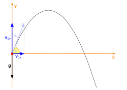
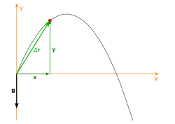
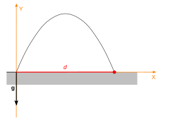
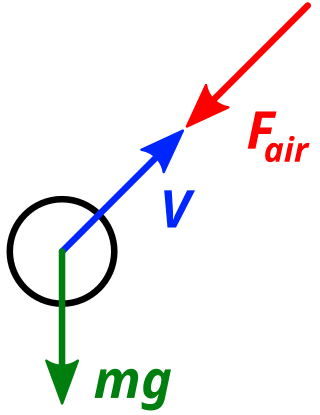
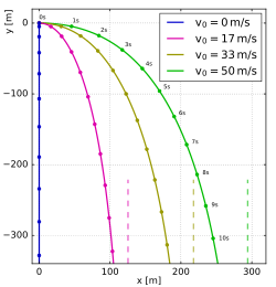
In physics, a projectile launched with specific initial conditions will have a range. It may be more predictable assuming a flat Earth with a uniform gravity field, and no air resistance. The horizontal ranges of a projectile are equal for two complementary angles of projection with the same velocity.

<span class="mw-page-title-main">Kepler orbit</span> Celestial orbit whose trajectory is a conic section in the orbital plane

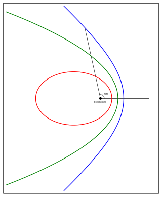
In celestial mechanics, a Kepler orbit is the motion of one body relative to another, as an ellipse, parabola, or hyperbola, which forms a two-dimensional orbital plane in three-dimensional space. A Kepler orbit can also form a straight line. It considers only the point-like gravitational attraction of two bodies, neglecting perturbations due to gravitational interactions with other objects, atmospheric drag, solar radiation pressure, a non-spherical central body, and so on. It is thus said to be a solution of a special case of the two-body problem, known as the Kepler problem. As a theory in classical mechanics, it also does not take into account the effects of general relativity. Keplerian orbits can be parametrized into six orbital elements in various ways.

In fluid dynamics, the Oseen equations describe the flow of a viscous and incompressible fluid at small Reynolds numbers, as formulated by Carl Wilhelm Oseen in 1910. Oseen flow is an improved description of these flows, as compared to Stokes flow, with the (partial) inclusion of convective acceleration.

<span class="mw-page-title-main">Lagrangian mechanics</span> Formulation of classical mechanics

In physics, Lagrangian mechanics is a formulation of classical mechanics founded on the stationary-action principle. It was introduced by the Italian-French mathematician and astronomer Joseph-Louis Lagrange in his presentation to the Turin Academy of Science in 1760 culminating in his 1788 grand opus, Mécanique analytique.

<span class="mw-page-title-main">Green's law</span> Equation describing evolution of waves in shallow water

In fluid dynamics, Green's law, named for 19th-century British mathematician George Green, is a conservation law describing the evolution of non-breaking, surface gravity waves propagating in shallow water of gradually varying depth and width. In its simplest form, for wavefronts and depth contours parallel to each other, it states:

In fluid dynamics, Taylor scraping flow is a type of two-dimensional corner flow occurring when one of the wall is sliding over the other with constant velocity, named after G. I. Taylor.

References

  1. Galileo Galilei, Two New Sciences , Leiden, 1638, p.249
  2. Nolte, David D., Galileo Unbound (Oxford University Press, 2018) pp. 39-63.
  3. Stewart, James; Clegg, Dan; Watson, Saleem (2021). Calculus: Early Transcendentals (Ninth ed.). Boston, MA: Cengage. p. 919. ISBN   978-1-337-61392-7.
  4. Tatum (2019). Classical Mechanics (PDF). pp. ch. 7.
  5. Stephen T. Thornton; Jerry B. Marion (2007). Classical Dynamics of Particles and Systems. Brooks/Cole. p. 59. ISBN   978-0-495-55610-7.
  6. Atam P. Arya; Atam Parkash Arya (September 1997). Introduction to Classical Mechanics. Prentice Hall Internat. p. 227. ISBN   978-0-13-906686-3.
  7. Rginald Cristian, Bernardo; Jose Perico, Esguerra; Jazmine Day, Vallejos; Jeff Jerard, Canda (2015). "Wind-influenced projectile motion". European Journal of Physics. 36 (2): 025016. Bibcode:2015EJPh...36b5016B. doi:10.1088/0143-0807/36/2/025016. S2CID   119601402.
  8. 1 2 3 Walter Greiner (2004). Classical Mechanics: Point Particles and Relativity. Springer Science & Business Media. p. 181. ISBN   0-387-95586-0.
  9. Ballistic Missile Defense, Glossary, v. 3.0, US Department of Defense, June 1997.