Quadtree

Last updated
Quadtree
Type Tree
Invented1974
Invented by Raphael Finkel and J.L. Bentley
Time complexity in big O notation
OperationAverageWorst case
Space complexity
A point-region quadtree with point data. Bucket capacity 1. Point quadtree.svg
A point-region quadtree with point data. Bucket capacity 1.
Quadtree compression of an image step by step. Left shows the compressed image with the tree bounding boxes while the right shows just the compressed image Quadtree compression of an image.gif
Quadtree compression of an image step by step. Left shows the compressed image with the tree bounding boxes while the right shows just the compressed image

A quadtree is a tree data structure in which each internal node has exactly four children. Quadtrees are the two-dimensional analog of octrees and are most often used to partition a two-dimensional space by recursively subdividing it into four quadrants or regions. The data associated with a leaf cell varies by application, but the leaf cell represents a "unit of interesting spatial information".

Contents

The subdivided regions may be square or rectangular, or may have arbitrary shapes. This data structure was named a quadtree by Raphael Finkel and J.L. Bentley in 1974. [1] A similar partitioning is also known as a Q-tree.

All forms of quadtrees share some common features:

A tree-pyramid (T-pyramid) is a "complete" tree; every node of the T-pyramid has four child nodes except leaf nodes; all leaves are on the same level, the level that corresponds to individual pixels in the image. The data in a tree-pyramid can be stored compactly in an array as an implicit data structure similar to the way a complete binary tree can be stored compactly in an array. [2]

Types

Quadtrees may be classified according to the type of data they represent, including areas, points, lines and curves. Quadtrees may also be classified by whether the shape of the tree is independent of the order in which data is processed. The following are common types of quadtrees.

Region quadtree

The region quadtree represents a partition of space in two dimensions by decomposing the region into four equal quadrants, subquadrants, and so on with each leaf node containing data corresponding to a specific subregion. Each node in the tree either has exactly four children, or has no children (a leaf node). The height of quadtrees that follow this decomposition strategy (i.e. subdividing subquadrants as long as there is interesting data in the subquadrant for which more refinement is desired) is sensitive to and dependent on the spatial distribution of interesting areas in the space being decomposed. The region quadtree is a type of trie.

A region quadtree with a depth of n may be used to represent an image consisting of 2n × 2n pixels, where each pixel value is 0 or 1. The root node represents the entire image region. If the pixels in any region are not entirely 0s or 1s, it is subdivided. In this application, each leaf node represents a block of pixels that are all 0s or all 1s. Note the potential savings in terms of space when these trees are used for storing images; images often have many regions of considerable size that have the same colour value throughout. Rather than store a big 2-D array of every pixel in the image, a quadtree can capture the same information potentially many divisive levels higher than the pixel-resolution sized cells that we would otherwise require. The tree resolution and overall size is bounded by the pixel and image sizes.

A region quadtree may also be used as a variable resolution representation of a data field. For example, the temperatures in an area may be stored as a quadtree, with each leaf node storing the average temperature over the subregion it represents.

Point quadtree

The point quadtree [3] is an adaptation of a binary tree used to represent two-dimensional point data. It shares the features of all quadtrees but is a true tree as the center of a subdivision is always on a point. It is often very efficient in comparing two-dimensional, ordered data points, usually operating in O(log n) time. Point quadtrees are worth mentioning for completeness, but they have been surpassed by k-d trees as tools for generalized binary search. [4]

Point quadtrees are constructed as follows. Given the next point to insert, we find the cell in which it lies and add it to the tree. The new point is added such that the cell that contains it is divided into quadrants by the vertical and horizontal lines that run through the point. Consequently, cells are rectangular but not necessarily square. In these trees, each node contains one of the input points.

Since the division of the plane is decided by the order of point-insertion, the tree's height is sensitive to and dependent on insertion order. Inserting in a "bad" order can lead to a tree of height linear in the number of input points (at which point it becomes a linked-list). If the point-set is static, pre-processing can be done to create a tree of balanced height.

Node structure for a point quadtree

A node of a point quadtree is similar to a node of a binary tree, with the major difference being that it has four pointers (one for each quadrant) instead of two ("left" and "right") as in an ordinary binary tree. Also a key is usually decomposed into two parts, referring to x and y coordinates. Therefore, a node contains the following information:

  • four pointers: quad[‘NW’], quad[‘NE’], quad[‘SW’], and quad[‘SE’]
  • point; which in turn contains:
    • key; usually expressed as x, y coordinates
    • value; for example a name

Point-region (PR) quadtree

Point-region (PR) quadtrees [5] [6] are very similar to region quadtrees. The difference is the type of information stored about the cells. In a region quadtree, a uniform value is stored that applies to the entire area of the cell of a leaf. The cells of a PR quadtree, however, store a list of points that exist within the cell of a leaf. As mentioned previously, for trees following this decomposition strategy the height depends on the spatial distribution of the points. Like the point quadtree, the PR quadtree may also have a linear height when given a "bad" set.

Edge quadtree

Edge quadtrees [7] [8] (much like PM quadtrees) are used to store lines rather than points. Curves are approximated by subdividing cells to a very fine resolution, specifically until there is a single line segment per cell. Near corners/vertices, edge quadtrees will continue dividing until they reach their maximum level of decomposition. This can result in extremely unbalanced trees which may defeat the purpose of indexing.

Polygonal map (PM) quadtree

The polygonal map quadtree (or PM Quadtree) is a variation of quadtree which is used to store collections of polygons that may be degenerate (meaning that they have isolated vertices or edges). [9] [10] A big difference between PM quadtrees and edge quadtrees is that the cell under consideration is not subdivided if the segments meet at a vertex in the cell.

There are three main classes of PM Quadtrees, which vary depending on what information they store within each black node. PM3 quadtrees can store any amount of non-intersecting edges and at most one point. PM2 quadtrees are the same as PM3 quadtrees except that all edges must share the same end point. Finally PM1 quadtrees are similar to PM2, but black nodes can contain a point and its edges or just a set of edges that share a point, but you cannot have a point and a set of edges that do not contain the point.

Compressed quadtrees

This section summarizes a subsection from a book by Sariel Har-Peled. [11]

If we were to store every node corresponding to a subdivided cell, we may end up storing a lot of empty nodes. We can cut down on the size of such sparse trees by only storing subtrees whose leaves have interesting data (i.e. "important subtrees"). We can actually cut down on the size even further. When we only keep important subtrees, the pruning process may leave long paths in the tree where the intermediate nodes have degree two (a link to one parent and one child). It turns out that we only need to store the node at the beginning of this path (and associate some meta-data with it to represent the removed nodes) and attach the subtree rooted at its end to . It is still possible for these compressed trees to have a linear height when given "bad" input points.

Although we trim a lot of the tree when we perform this compression, it is still possible to achieve logarithmic-time search, insertion, and deletion by taking advantage of Z-order curves. The Z-order curve maps each cell of the full quadtree (and hence even the compressed quadtree) in time to a one-dimensional line (and maps it back in time too), creating a total order on the elements. Therefore, we can store the quadtree in a data structure for ordered sets (in which we store the nodes of the tree).

We must state a reasonable assumption before we continue: we assume that given two real numbers expressed as binary, we can compute in time the index of the first bit in which they differ. We also assume that we can compute in time the lowest common ancestor of two points/cells in the quadtree and establish their relative Z-ordering, and we can compute the floor function in time.

With these assumptions, point location of a given point (i.e. determining the cell that would contain ), insertion, and deletion operations can all be performed in time (i.e. the time it takes to do a search in the underlying ordered set data structure).

To perform a point location for (i.e. find its cell in the compressed tree):

  1. Find the existing cell in the compressed tree that comes before in the Z-order. Call this cell .
  2. If , return .
  3. Else, find what would have been the lowest common ancestor of the point and the cell in an uncompressed quadtree. Call this ancestor cell .
  4. Find the existing cell in the compressed tree that comes before in the Z-order and return it.

Without going into specific details, to perform insertions and deletions we first do a point location for the thing we want to insert/delete, and then insert/delete it. Care must be taken to reshape the tree as appropriate, creating and removing nodes as needed.

Some common uses of quadtrees

Image processing using quadtrees

Quadtrees, particularly the region quadtree, have lent themselves well to image processing applications. We will limit our discussion to binary image data, though region quadtrees and the image processing operations performed on them are just as suitable for colour images. [4] [16]

Image union / intersection

One of the advantages of using quadtrees for image manipulation is that the set operations of union and intersection can be done simply and quickly. [4] [17] [18] [19] [20] Given two binary images, the image union (also called overlay) produces an image wherein a pixel is black if either of the input images has a black pixel in the same location. That is, a pixel in the output image is white only when the corresponding pixel in both input images is white, otherwise the output pixel is black. Rather than do the operation pixel by pixel, we can compute the union more efficiently by leveraging the quadtree's ability to represent multiple pixels with a single node. For the purposes of discussion below, if a subtree contains both black and white pixels we will say that the root of that subtree is coloured grey.

The algorithm works by traversing the two input quadtrees ( and ) while building the output quadtree . Informally, the algorithm is as follows. Consider the nodes and corresponding to the same region in the images.

While this algorithm works, it does not by itself guarantee a minimally sized quadtree. For example, consider the result if we were to union a checkerboard (where every tile is a pixel) of size with its complement. The result is a giant black square which should be represented by a quadtree with just the root node (coloured black), but instead the algorithm produces a full 4-ary tree of depth . To fix this, we perform a bottom-up traversal of the resulting quadtree where we check if the four children nodes have the same colour, in which case we replace their parent with a leaf of the same colour. [4]

The intersection of two images is almost the same algorithm. One way to think about the intersection of the two images is that we are doing a union with respect to the white pixels. As such, to perform the intersection we swap the mentions of black and white in the union algorithm.

Connected component labelling

Consider two neighbouring black pixels in a binary image. They are adjacent if they share a bounding horizontal or vertical edge. In general, two black pixels are connected if one can be reached from the other by moving only to adjacent pixels (i.e. there is a path of black pixels between them where each consecutive pair is adjacent). Each maximal set of connected black pixels is a connected component. Using the quadtree representation of images, Samet [21] showed how we can find and label these connected components in time proportional to the size of the quadtree. [4] [22] This algorithm can also be used for polygon colouring.

The algorithm works in three steps:

To simplify the discussion, let us assume the children of a node in the quadtree follow the Z-order (SW, NW, SE, NE). Since we can count on this structure, for any cell we know how to navigate the quadtree to find the adjacent cells in the different levels of the hierarchy.

Step one is accomplished with a post-order traversal of the quadtree. For each black leaf we look at the node or nodes representing cells that are Northern neighbours and Eastern neighbours (i.e. the Northern and Eastern cells that share edges with the cell of ). Since the tree is organized in Z-order, we have the invariant that the Southern and Western neighbours have already been taken care of and accounted for. Let the Northern or Eastern neighbour currently under consideration be . If represents black pixels:

Step two can be accomplished using the union-find data structure. [23] We start with each unique label as a separate set. For every equivalence relation noted in the first step, we union the corresponding sets. Afterwards, each distinct remaining set will be associated with a distinct connected component in the image.

Step three performs another post-order traversal. This time, for each black node we use the union-find's find operation (with the old label of ) to find and assign its new label (associated with the connected component of which is part).

Mesh generation using quadtrees

This section summarizes a chapter from a book by Har-Peled and de Berg et al. [24] [25]

Mesh generation is essentially the triangulation of a point set for which further processing may be performed. As such, it is desirable for the resulting triangulation to have certain properties (like non-uniformity, triangles that are not "too skinny", large triangles in sparse areas and small triangles in dense ones, etc.) to make further processing quicker and less error-prone. Quadtrees built on the point set can be used to create meshes with these desired properties.

A balanced leaf has at most one corner in a side. Fig-mesh-gen-balanced-leaves.svg
A balanced leaf has at most one corner in a side.

Consider a leaf of the quadtree and its corresponding cell . We say is balanced (for mesh generation) if the cell's sides are intersected by the corner points of neighbouring cells at most once on each side. This means that the quadtree levels of leaves adjacent to differ by at most one from the level of . When this is true for all leaves, we say the whole quadtree is balanced (for mesh generation).

Consider the cell and the neighbourhood of same-sized cells centred at . We call this neighbourhood the extended cluster. We say the quadtree is well-balanced if it is balanced, and for every leaf that contains a point of the point set, its extended cluster is also in the quadtree and the extended cluster contains no other point of the point set.

Creating the mesh is done as follows:

  1. Build a quadtree on the input points.
  2. Ensure the quadtree is balanced. For every leaf, if there is a neighbour that is too large, subdivide the neighbour. This is repeated until the tree is balanced. We also make sure that for a leaf with a point in it, the nodes for each leaf's extended cluster are in the tree.
  3. For every leaf node that contains a point, if the extended cluster contains another point, we further subdivide the tree and rebalance as necessary. If we needed to subdivide, for each child of we ensure the nodes of 's extended cluster are in the tree (and re-balance as required).
  4. Repeat the previous step until the tree is well-balanced.
  5. Transform the quadtree into a triangulation.

We consider the corner points of the tree cells as vertices in our triangulation. Before the transformation step we have a bunch of boxes with points in some of them. The transformation step is done in the following manner: for each point, warp the closest corner of its cell to meet it and triangulate the resulting four quadrangles to make "nice" triangles (the interested reader is referred to chapter 12 of Har-Peled [24] for more details on what makes "nice" triangles).

The remaining squares are triangulated according to some simple rules. For each regular square (no points within and no corner points in its sides), introduce the diagonal. Due to the way in which we separated points with the well-balancing property, no square with a corner intersecting a side is one that was warped. As such, we can triangulate squares with intersecting corners as follows. If there is one intersected side, the square becomes three triangles by adding the long diagonals connecting the intersection with opposite corners. If there are four intersected sides, we split the square in half by adding an edge between two of the four intersections, and then connect these two endpoints to the remaining two intersection points. For the other squares, we introduce a point in the middle and connect it to all four corners of the square as well as each intersection point.

At the end of it all, we have a nice triangulated mesh of our point set built from a quadtree.

Pseudocode

The following pseudo code shows one means of implementing a quadtree which handles only points. There are other approaches available.

Prerequisites

It is assumed these structures are used.

// Simple coordinate object to represent points and vectorsstruct XY {     float x;     float y;      function __construct(float _x, float _y) {...} }  // Axis-aligned bounding box with half dimension and centerstruct AABB {     XY center;     float halfDimension;      function __construct(XY _center, float _halfDimension) {...}     function containsPoint(XY point) {...}     function intersectsAABB(AABB other) {...} }

QuadTree class

This class represents both one quad tree and the node where it is rooted.

class QuadTree {     // Arbitrary constant to indicate how many elements can be stored in this quad tree nodeconstant int QT_NODE_CAPACITY = 4;      // Axis-aligned bounding box stored as a center with half-dimensions// to represent the boundaries of this quad treeAABB boundary;      // Points in this quad tree nodeArray of XY [size = QT_NODE_CAPACITY] points;      // ChildrenQuadTree* northWest;     QuadTree* northEast;     QuadTree* southWest;     QuadTree* southEast;      // Methodsfunction __construct(AABB _boundary) {...}     function insert(XY p) {...}     function subdivide() {...} // create four children that fully divide this quad into four quads of equal areafunction queryRange(AABB range) {...} }

Insertion

The following method inserts a point into the appropriate quad of a quadtree, splitting if necessary.

class QuadTree {     ...        // Insert a point into the QuadTreefunction insert(XY p)     {         // Ignore objects that do not belong in this quad treeif (!boundary.containsPoint(p))             returnfalse; // object cannot be added// If there is space in this quad tree and if doesn't have subdivisions, add the object hereif (points.size < QT_NODE_CAPACITY && northWest == null)         {             points.append(p);             returntrue;         }              // Otherwise, subdivide and then add the point to whichever node will accept itif (northWest == null)             subdivide();         // We have to add the points/data contained in this quad array to the new quads if we only want// the last node to hold the dataif (northWest->insert(p)) returntrue;         if (northEast->insert(p)) returntrue;         if (southWest->insert(p)) returntrue;         if (southEast->insert(p)) returntrue;              // Otherwise, the point cannot be inserted for some unknown reason (this should never happen)returnfalse;     } }

Query range

The following method finds all points contained within a range.

class QuadTree {     ...        // Find all points that appear within a rangefunction queryRange(AABB range)     {         // Prepare an array of resultsArray of XY pointsInRange;              // Automatically abort if the range does not intersect this quadif (!boundary.intersectsAABB(range))             return pointsInRange; // empty list// Check objects at this quad levelfor (int p = 0; p < points.size; p++)         {             if (range.containsPoint(points[p]))                 pointsInRange.append(points[p]);         }              // Terminate here, if there are no childrenif (northWest == null)             return pointsInRange;              // Otherwise, add the points from the children         pointsInRange.appendArray(northWest->queryRange(range));         pointsInRange.appendArray(northEast->queryRange(range));         pointsInRange.appendArray(southWest->queryRange(range));         pointsInRange.appendArray(southEast->queryRange(range));              return pointsInRange;     } }

See also

Related Research Articles

<span class="mw-page-title-main">AVL tree</span> Self-balancing binary search tree

In computer science, an AVL tree is a self-balancing binary search tree. In an AVL tree, the heights of the two child subtrees of any node differ by at most one; if at any time they differ by more than one, rebalancing is done to restore this property. Lookup, insertion, and deletion all take O(log n) time in both the average and worst cases, where is the number of nodes in the tree prior to the operation. Insertions and deletions may require the tree to be rebalanced by one or more tree rotations.

<span class="mw-page-title-main">Binary search tree</span> Rooted binary tree data structure

In computer science, a binary search tree (BST), also called an ordered or sorted binary tree, is a rooted binary tree data structure with the key of each internal node being greater than all the keys in the respective node's left subtree and less than the ones in its right subtree. The time complexity of operations on the binary search tree is linear with respect to the height of the tree.

<span class="mw-page-title-main">Binary tree</span> Limited form of tree data structure

In computer science, a binary tree is a tree data structure in which each node has at most two children, referred to as the left child and the right child. That is, it is a k-ary tree with k = 2. A recursive definition using set theory is that a binary tree is a tuple (L, S, R), where L and R are binary trees or the empty set and S is a singleton set containing the root.

In computer science, a B-tree is a self-balancing tree data structure that maintains sorted data and allows searches, sequential access, insertions, and deletions in logarithmic time. The B-tree generalizes the binary search tree, allowing for nodes with more than two children. Unlike other self-balancing binary search trees, the B-tree is well suited for storage systems that read and write relatively large blocks of data, such as databases and file systems.

In computer science, a red–black tree is a specialised binary search tree data structure noted for fast storage and retrieval of ordered information, and a guarantee that operations will complete within a known time. Compared to other self-balancing binary search trees, the nodes in a red-black tree hold an extra bit called "color" representing "red" and "black" which is used when re-organising the tree to ensure that it is always approximately balanced.

<span class="mw-page-title-main">Binary heap</span> Variant of heap data structure

A binary heap is a heap data structure that takes the form of a binary tree. Binary heaps are a common way of implementing priority queues. The binary heap was introduced by J. W. J. Williams in 1964, as a data structure for heapsort.

<span class="mw-page-title-main">Treap</span> Random search tree data structure

In computer science, the treap and the randomized binary search tree are two closely related forms of binary search tree data structures that maintain a dynamic set of ordered keys and allow binary searches among the keys. After any sequence of insertions and deletions of keys, the shape of the tree is a random variable with the same probability distribution as a random binary tree; in particular, with high probability its height is proportional to the logarithm of the number of keys, so that each search, insertion, or deletion operation takes logarithmic time to perform.

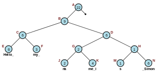
In computer science, a 2–3 tree is a tree data structure, where every node with children has either two children (2-node) and one data element or three children (3-node) and two data elements. A 2–3 tree is a B-tree of order 3. Nodes on the outside of the tree have no children and one or two data elements. 2–3 trees were invented by John Hopcroft in 1970.

<span class="mw-page-title-main">Octree</span> Tree data structure in which each internal node has exactly eight children, to partition a 3D space

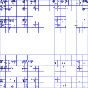
An octree is a tree data structure in which each internal node has exactly eight children. Octrees are most often used to partition a three-dimensional space by recursively subdividing it into eight octants. Octrees are the three-dimensional analog of quadtrees. The word is derived from oct + tree. Octrees are often used in 3D graphics and 3D game engines.

<span class="mw-page-title-main">R-tree</span> Data structures used in spatial indexing

R-trees are tree data structures used for spatial access methods, i.e., for indexing multi-dimensional information such as geographical coordinates, rectangles or polygons. The R-tree was proposed by Antonin Guttman in 1984 and has found significant use in both theoretical and applied contexts. A common real-world usage for an R-tree might be to store spatial objects such as restaurant locations or the polygons that typical maps are made of: streets, buildings, outlines of lakes, coastlines, etc. and then find answers quickly to queries such as "Find all museums within 2 km of my current location", "retrieve all road segments within 2 km of my location" or "find the nearest gas station". The R-tree can also accelerate nearest neighbor search for various distance metrics, including great-circle distance.

<span class="mw-page-title-main">Rope (data structure)</span> Data structure for storing strings

In computer programming, a rope, or cord, is a data structure composed of smaller strings that is used to efficiently store and manipulate a very long string. For example, a text editing program may use a rope to represent the text being edited, so that operations such as insertion, deletion, and random access can be done efficiently.

<span class="mw-page-title-main">T-tree</span> Data structure in computer science

In computer science a T-tree is a type of binary tree data structure that is used by main-memory databases, such as Datablitz, eXtremeDB, MySQL Cluster, Oracle TimesTen and MobileLite.

In computer science, a scapegoat tree is a self-balancing binary search tree, invented by Arne Andersson in 1989 and again by Igal Galperin and Ronald L. Rivest in 1993. It provides worst-case lookup time and amortized insertion and deletion time.

In computer science, an interval tree is a tree data structure to hold intervals. Specifically, it allows one to efficiently find all intervals that overlap with any given interval or point. It is often used for windowing queries, for instance, to find all roads on a computerized map inside a rectangular viewport, or to find all visible elements inside a three-dimensional scene. A similar data structure is the segment tree.

<i>k</i>-d tree Multidimensional search tree for points in k dimensional space

In computer science, a k-d tree is a space-partitioning data structure for organizing points in a k-dimensional space. K-dimensional is that which concerns exactly k orthogonal axes or a space of any number of dimensions. k-d trees are a useful data structure for several applications, such as:

A vantage-point tree is a metric tree that segregates data in a metric space by choosing a position in the space and partitioning the data points into two parts: those points that are nearer to the vantage point than a threshold, and those points that are not. By recursively applying this procedure to partition the data into smaller and smaller sets, a tree data structure is created where neighbors in the tree are likely to be neighbors in the space.

<span class="mw-page-title-main">Segment tree</span> Computer science data structure

In computer science, the segment tree is a data structure used for storing information about intervals or segments. It allows querying which of the stored segments contain a given point. A similar data structure is the interval tree.

In computer science, a range tree is an ordered tree data structure to hold a list of points. It allows all points within a given range to be reported efficiently, and is typically used in two or higher dimensions. Range trees were introduced by Jon Louis Bentley in 1979. Similar data structures were discovered independently by Lueker, Lee and Wong, and Willard. The range tree is an alternative to the k-d tree. Compared to k-d trees, range trees offer faster query times of but worse storage of , where n is the number of points stored in the tree, d is the dimension of each point and k is the number of points reported by a given query.

<span class="mw-page-title-main">Cartesian tree</span> Binary tree derived from a sequence of numbers

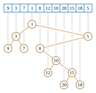
In computer science, a Cartesian tree is a binary tree derived from a sequence of distinct numbers. To construct the Cartesian tree, set its root to be the minimum number in the sequence, and recursively construct its left and right subtrees from the subsequences before and after this number. It is uniquely defined as a min-heap whose symmetric (in-order) traversal returns the original sequence.

<span class="mw-page-title-main">VC-6</span> A video coding format

SMPTE ST 2117-1, informally known as VC-6, is a video coding format.

References

Surveys by Aluru [4] and Samet [22] [16] give a nice overview of quadtrees.

Notes

  1. Finkel, R. A.; Bentley, J. L. (1974). "Quad trees a data structure for retrieval on composite keys". Acta Informatica. 4 (1): 1–9. doi:10.1007/BF00288933. S2CID   33019699 . Retrieved 6 November 2019.
  2. Milan Sonka, Vaclav Hlavac, Roger Boyle. "Image Processing, Analysis, and Machine Vision". 2014. p. 108-109.
  3. Finkel, R. A.; Bentley, J. L. (1974). "Quad Trees A Data Structure for Retrieval on Composite Keys". Acta Informatica. 4. Springer-Verlag: 1–9. doi:10.1007/bf00288933. S2CID   33019699.
  4. 1 2 3 4 5 6 Aluru, S. (2004). "Quadtrees and octrees". In D. Mehta and S. Sahni (ed.). Handbook of Data Structures and Applications. Chapman and Hall/CRC. pp. 19-1 -- 19-26. ISBN   9781584884354.
  5. Orenstein, J. A. (1982). "Multidimensional tries used for associative searching". Information Processing Letters. 14 (4). Elsevier: 150–157. doi:10.1016/0020-0190(82)90027-8.
  6. Samet, H. (1984). "The quadtree and related hierarchical data structures" (PDF). ACM Computing Surveys. 16 (2). ACM: 187–260. doi:10.1145/356924.356930. S2CID   10319214.
  7. Warnock, J. E. (1969). "A hidden surface algorithm for computer generated halftone pictures". Computer Science Department, University of Utah. TR 4-15.
  8. Schneier, M. (1981). "Two hierarchical linear feature representations: edge pyramids and edge quadtrees". Computer Graphics and Image Processing. 17 (3). Elsevier: 211–224. doi:10.1016/0146-664X(81)90002-2.
  9. Hanan Samet and Robert Webber. "Storing a Collection of Polygons Using Quadtrees". ACM Transactions on Graphics July 1985: 182-222. InfoLAB. Web. 23 March 2012
  10. Nelson, R. C.; Samet, H. (1986). "A consistent hierarchical representation for vector data". ACM SIGGRAPH Computer Graphics. 20 (4): 197–206. doi: 10.1145/15886.15908 .
  11. Har-Peled, S. (2011). "Quadtrees - Hierarchical Grids". Geometric approximation algorithms. Mathematical Surveys and Monographs Vol. 173, American mathematical society.
  12. Wanta, Damian; Smolik, Waldemar T.; Kryszyn, Jacek; Wróblewski, Przemysław; Midura, Mateusz (2021). "A Finite Volume Method using a Quadtree Non-Uniform Structured Mesh for Modeling in Electrical Capacitance Tomography". Proceedings of the National Academy of Sciences, India Section A. 92 (3): 443–452. doi: 10.1007/s40010-021-00748-7 . S2CID   244224810.
  13. Sestoft, Peter (2014). Spreadsheet Implementation Technology: Basics and Extensions. The MIT Press. pp. 60–63. ISBN   9780262526647.
  14. Tomas G. Rokicki (2006-04-01). "An Algorithm for Compressing Space and Time" . Retrieved 2009-05-20.
  15. Henning Eberhardt, Vesa Klumpp, Uwe D. Hanebeck, Density Trees for Efficient Nonlinear State Estimation, Proceedings of the 13th International Conference on Information Fusion, Edinburgh, United Kingdom, July, 2010.
  16. 1 2 Samet, H. (1989). "Hierarchical spatial data structures". Symposium on Large Spatial Databases: 191–212.
  17. Hunter, G. M. (1978). Efficient Computation and Data Structures for Graphics. Ph.D. dissertation, Department of Electrical Engineering and Computer Science, Princeton University.
  18. Hunter, G. M.; Steiglitz, K. (1979). "Operations on images using quad trees". IEEE Transactions on Pattern Analysis and Machine Intelligence. 2 (2): 145–153. doi:10.1109/tpami.1979.4766900. PMID   21868843. S2CID   2544535.
  19. Schneier, M. (1981). "Calculations of geometric properties using quadtrees". Computer Graphics and Image Processing. 16 (3): 296–302. doi:10.1016/0146-664X(81)90042-3.
  20. Mehta, Dinesh (2007). Handbook of Data Structures and Applications. Chapman and Hall/CRC Press. p. 397.
  21. Samet, H. (1981). "Connected component labeling using quadtrees". Journal of the ACM. 28 (3): 487–501. CiteSeerX   10.1.1.77.2573 . doi:10.1145/322261.322267. S2CID   17485118.
  22. 1 2 Samet, H. (1988). "An overview of quadtrees, octrees, and related hierarchical data structures". In Earnshaw, R. A. (ed.). Theoretical Foundations of Computer Graphics and CAD. Springer-Verlag. pp. 51–68.
  23. Tarjan, R. E. (1975). "Efficiency of a good but not linear set union algorithm" (PDF). Journal of the ACM. 22 (2): 215–225. doi:10.1145/321879.321884. hdl: 1813/5942 . S2CID   11105749.
  24. 1 2 Har-Peled, S. (2011). "Good Triangulations and Meshing". Geometric approximation algorithms. Mathematical Surveys and Monographs Vol. 173, American mathematical society.
  25. de Berg, M.; Cheong, O.; van Kreveld, M.; Overmars, M. H. (2008). "Quadtrees Non-Uniform Mesh Generation". Computational Geometry Algorithms and Applications (3rd ed.). Springer-Verlag.

General references

  1. Raphael Finkel and J.L. Bentley (1974). "Quad Trees: A Data Structure for Retrieval on Composite Keys". Acta Informatica. 4 (1): 1–9. doi:10.1007/BF00288933. S2CID   33019699.
  2. Mark de Berg, Marc van Kreveld, Mark Overmars, and Otfried Schwarzkopf (2000). Computational Geometry (2nd revised ed.). Springer-Verlag. ISBN   3-540-65620-0.{{cite book}}: CS1 maint: multiple names: authors list (link) Chapter 14: Quadtrees: pp. 291–306.
  3. Samet, Hanan; Webber, Robert (July 1985). "Storing a Collection of Polygons Using Quadtrees" (PDF). Retrieved 23 March 2012.