
Depth-first search (DFS) is an algorithm for traversing or searching tree or graph data structures. The algorithm starts at the root node and explores as far as possible along each branch before backtracking.
This is a glossary of graph theory. Graph theory is the study of graphs, systems of nodes or vertices connected in pairs by lines or edges.

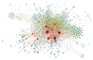
Graph drawing is an area of mathematics and computer science combining methods from geometric graph theory and information visualization to derive two-dimensional depictions of graphs arising from applications such as social network analysis, cartography, linguistics, and bioinformatics.

In order theory, a Hasse diagram is a type of mathematical diagram used to represent a finite partially ordered set, in the form of a drawing of its transitive reduction. Concretely, for a partially ordered set (S, ≤) one represents each element of S as a vertex in the plane and draws a line segment or curve that goes upward from x to y whenever y covers x . These curves may cross each other but must not touch any vertices other than their endpoints. Such a diagram, with labeled vertices, uniquely determines its partial order.
Force-directed graph drawing algorithms are a class of algorithms for drawing graphs in an aesthetically-pleasing way. Their purpose is to position the nodes of a graph in two-dimensional or three-dimensional space so that all the edges are of more or less equal length and there are as few crossing edges as possible, by assigning forces among the set of edges and the set of nodes, based on their relative positions, and then using these forces either to simulate the motion of the edges and nodes or to minimize their energy.
In mathematics, topological graph theory is a branch of graph theory. It studies the embedding of graphs in surfaces, spatial embeddings of graphs, and graphs as topological spaces. It also studies immersions of graphs.

In the mathematical discipline of graph theory, the dual graph of a plane graph G is a graph that has a vertex for each face of G. The dual graph has an edge for each pair of faces in G that are separated from each other by an edge, and a self-loop when the same face appears on both sides of an edge. Thus, each edge e of G has a corresponding dual edge, whose endpoints are the dual vertices corresponding to the faces on either side of e. The definition of the dual depends on the choice of embedding of the graph G, so it is a property of plane graphs rather than planar graphs. For planar graphs generally, there may be multiple dual graphs, depending on the choice of planar embedding of the graph.

In graph theory, a biconnected component is a maximal biconnected subgraph. Any connected graph decomposes into a tree of biconnected components called the block-cut tree of the graph. The blocks are attached to each other at shared vertices called cut vertices or separating vertices or articulation points. Specifically, a cut vertex is any vertex whose removal increases the number of connected components.
A program structure tree (PST) is a hierarchical diagram that displays the nesting relationship of single-entry single-exit (SESE) fragments/regions, showing the organization of a computer program. Nodes in this tree represent SESE regions of the program, while edges represent nesting regions. The PST is defined for all control flow graphs.
Planarity is a puzzle computer game by John Tantalo, based on a concept by Mary Radcliffe at Western Michigan University. The name comes from the concept of planar graphs in graph theory; these are graphs that can be embedded in the Euclidean plane so that no edges intersect. By Fáry's theorem, if a graph is planar, it can be drawn without crossings so that all of its edges are straight line segments. In the planarity game, the player is presented with a circular layout of a planar graph, with all the vertices placed on a single circle and with many crossings. The goal for the player is to eliminate all of the crossings and construct a straight-line embedding of the graph by moving the vertices one by one into better positions.
In graph theory, the planarity testing problem is the algorithmic problem of testing whether a given graph is a planar graph. This is a well-studied problem in computer science for which many practical algorithms have emerged, many taking advantage of novel data structures. Most of these methods operate in O(n) time, where n is the number of edges in the graph, which is asymptotically optimal. Rather than just being a single Boolean value, the output of a planarity testing algorithm may be a planar graph embedding, if the graph is planar, or an obstacle to planarity such as a Kuratowski subgraph if it is not.
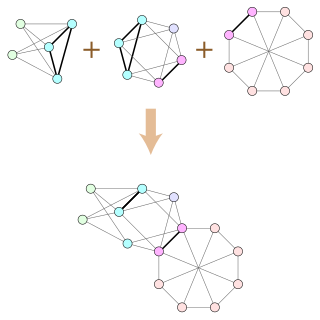
In graph theory, a branch of mathematics, a clique-sum is a way of combining two graphs by gluing them together at a clique, analogous to the connected sum operation in topology. If two graphs G and H each contain cliques of equal size, the clique-sum of G and H is formed from their disjoint union by identifying pairs of vertices in these two cliques to form a single shared clique, and then possibly deleting some of the clique edges. A k-clique-sum is a clique-sum in which both cliques have at most k vertices. One may also form clique-sums and k-clique-sums of more than two graphs, by repeated application of the two-graph clique-sum operation.
In graph theory, the planar separator theorem is a form of isoperimetric inequality for planar graphs, that states that any planar graph can be split into smaller pieces by removing a small number of vertices. Specifically, the removal of vertices from an n-vertex graph can partition the graph into disjoint subgraphs each of which has at most vertices.

In graph theory, a branch of mathematics, an apex graph is a graph that can be made planar by the removal of a single vertex. The deleted vertex is called an apex of the graph. It is an apex, not the apex because an apex graph may have more than one apex; for example, in the minimal nonplanar graphs K5 or K3,3, every vertex is an apex. The apex graphs include graphs that are themselves planar, in which case again every vertex is an apex. The null graph is also counted as an apex graph even though it has no vertex to remove.

In graph drawing, the angular resolution of a drawing of a graph is the sharpest angle formed by any two edges that meet at a common vertex of the drawing.
In topological graph theory, a 1-planar graph is a graph that can be drawn in the Euclidean plane in such a way that each edge has at most one crossing point, where it crosses a single additional edge. If a 1-planar graph, one of the most natural generalizations of planar graphs, is drawn that way, the drawing is called a 1-plane graph or 1-planar embedding of the graph.
In graph theory, a bipolar orientation or st-orientation of an undirected graph is an assignment of a direction to each edge that causes the graph to become a directed acyclic graph with a single source s and a single sink t, and an st-numbering of the graph is a topological ordering of the resulting directed acyclic graph.
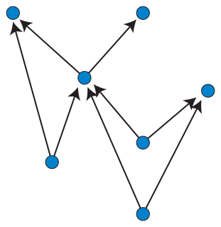
In graph drawing, an upward planar drawing of a directed acyclic graph is an embedding of the graph into the Euclidean plane, in which the edges are represented as non-crossing monotonic upwards curves. That is, the curve representing each edge should have the property that every horizontal line intersects it in at most one point, and no two edges may intersect except at a shared endpoint. In this sense, it is the ideal case for layered graph drawing, a style of graph drawing in which edges are monotonic curves that may cross, but in which crossings are to be minimized.
In the mathematical field of graph theory, planarization is a method of extending graph drawing methods from planar graphs to graphs that are not planar, by embedding the non-planar graphs within a larger planar graph.
In graph drawing, the area used by a drawing is a commonly used way of measuring its quality.
