Quantile-parameterized distribution

Last updated

A quantile-parameterized distribution (QPD) is a probability distributions that is directly parameterized by data. They were created to meet the need for easy-to-use continuous probability distributions flexible enough to represent a wide range of uncertainties, such as those commonly encountered in business, economics, engineering, and science. Because QPDs are directly parameterized by data, they have the practical advantage of avoiding the intermediate step of parameter estimation, a time-consuming process that typically requires non-linear iterative methods to estimate probability-distribution parameters from data. Some QPDs have virtually unlimited shape flexibility and closed-form moments as well.

Contents

History

The development of quantile-parameterized distributions was inspired by the practical need for flexible continuous probability distributions that are easy to fit to data. Historically, the Pearson [1] and Johnson [2] [3] families of distributions have been used when shape flexibility is needed. That is because both families can match the first four moments (mean, variance, skewness, and kurtosis) of any data set. In many cases, however, these distributions are either difficult to fit to data or not flexible enough to fit the data appropriately.

For example, the beta distribution is a flexible Pearson distribution that is frequently used to model percentages of a population. However, if the characteristics of this population are such that the desired cumulative distribution function (CDF) should run through certain specific CDF points, there may be no beta distribution that meets this need. Because the beta distribution has only two shape parameters, it cannot, in general, match even three specified CDF points. Moreover, the beta parameters that best fit such data can be found only by nonlinear iterative methods.

Practitioners of decision analysis, needing distributions easily parameterized by three or more CDF points (e.g., because such points were specified as the result of an expert-elicitation process), originally invented quantile-parameterized distributions for this purpose. Keelin and Powley (2011) [4] provided the original definition. Subsequently, Keelin (2016) [5] developed the metalog distributions, a family of quantile-parameterized distributions that has virtually unlimited shape flexibility, simple equations, and closed-form moments.

Definition

Keelin and Powley [4] define a quantile-parameterized distribution as one whose quantile function (inverse CDF) can be written in the form

where

and the functions are continuously differentiable and linearly independent basis functions. Here, essentially, and are the lower and upper bounds (if they exist) of a random variable with quantile function . These distributions are called quantile-parameterized because for a given set of quantile pairs , where , and a set of basis functions , the coefficients can be determined by solving a set of linear equations. [4] If one desires to use more quantile pairs than basis functions, then the coefficients can be chosen to minimize the sum of squared errors between the stated quantiles and . Keelin and Powley [4] illustrate this concept for a specific choice of basis functions that is a generalization of quantile function of the normal distribution, , for which the mean and standard deviation are linear functions of cumulative probability :

The result is a four-parameter distribution that can be fit to a set of four quantile/probability pairs exactly, or to any number of such pairs by linear least squares. Keelin and Powley [4] call this the Simple Q-Normal distribution. Some skewed and symmetric Simple Q-Normal PDFs are shown in the figures below.

Symmetric Simple Q-Normal PDFs SymmetricSimpleQNormalFree.png
Symmetric Simple Q-Normal PDFs
Skewed Simple Q-Normal PDFs Skewed Simple Q Normal Distributions.png
Skewed Simple Q-Normal PDFs

Properties

QPD’s that meet Keelin and Powley’s definition have the following properties.

Probability density function

Differentiating with respect to yields . The reciprocal of this quantity, , is the probability density function (PDF)

where . Note that this PDF is expressed as a function of cumulative probability rather than . To plot it, as shown in the figures, vary parametrically. Plot on the horizontal axis and on the vertical axis.

Feasibility

A function of the form of is a feasible probability distribution if and only if for all . [4] This implies a feasibility constraint on the set of coefficients :

for all

In practical applications, feasibility must generally be checked rather than assumed.

Convexity

A QPD’s set of feasible coefficients for all is convex. Because convex optimization requires convex feasible sets, this property simplifies optimization applications involving QPDs.

Fitting to data

The coefficients can be determined from data by linear least squares. Given data points that are intended to characterize the CDF of a QPD, and matrix whose elements consist of , then, so long as is invertible, coefficients' column vector can be determined as , where and column vector . If , this equation reduces to , where the resulting CDF runs through all data points exactly. An alternate method, implemented as a linear program, determines the coefficients by minimizing the sum of absolute distances between the CDF and the data subject to feasibility constraints. [6]

Shape flexibility

A QPD with terms, where , has shape parameters. Thus, QPDs can be far more flexible than the Pearson distributions, which have at most two shape parameters. For example, ten-term metalog distributions parameterized by 105 CDF points from 30 traditional source distributions (including normal, student-t, lognormal, gamma, beta, and extreme value) have been shown to approximate each such source distribution within a K–S distance of 0.001 or less. [7]

Transformations

QPD transformations are governed by a general property of quantile functions: for any quantile function and increasing function is a quantile function. [8] For example, the quantile function of the normal distribution, , is a QPD by the Keelin and Powley definition. The natural logarithm, , is an increasing function, so is the quantile function of the lognormal distribution with lower bound . Importantly, this transformation converts an unbounded QPD into a semi-bounded QPD. Similarly, applying this log transformation to the unbounded metalog distribution [9] yields the semi-bounded (log) metalog distribution; [10] likewise, applying the logit transformation, , yields the bounded (logit) metalog distribution [10] with lower and upper bounds and , respectively. Moreover, by considering to be distributed, where is any QPD that meets Keelin and Powley’s definition, the transformed variable maintains the above properties of feasibility, convexity, and fitting to data. Such transformed QPDs have greater shape flexibility than the underlying , which has shape parameters; the log transformation has shape parameters, and the logit transformation has shape parameters. Moreover, such transformed QPDs share the same set of feasible coefficients as the underlying untransformed QPD. [11]


Moments

The moment of a QPD is: [4]

Whether such moments exist in closed form depends on the choice of QPD basis functions . The unbounded metalog distribution and polynomial QPDs are examples of QPDs for which moments exist in closed form as functions of the coefficients .

Simulation

Since the quantile function is expressed in closed form, Keelin and Powley QPDs facilitate Monte Carlo simulation. Substituting in uniformly distributed random samples of produces random samples of in closed form, thereby eliminating the need to invert a CDF expressed as .

The following probability distributions are QPDs according to Keelin and Powley’s definition:

Like the SPT metalog distributions, the Johnson Quantile-Parameterized Distributions [14] [15] (JQPDs) are parameterized by three quantiles. JQPDs do not meet Keelin and Powley’s QPD definition, but rather have their own properties. JQPDs are feasible for all SPT parameter sets that are consistent with the rules of probability.

Applications

The original applications of QPDs were by decision analysts wishing to conveniently convert expert-assessed quantiles (e.g., 10th, 50th, and 90th quantiles) into smooth continuous probability distributions. QPDs have also been used to fit output data from simulations in order to represent those outputs (both CDFs and PDFs) as closed-form continuous distributions. [16] Used in this way, they are typically more stable and smoother than histograms. Similarly, since QPDs can impose fewer shape constraints than traditional distributions, they have been used to fit a wide range of empirical data in order to represent those data sets as continuous distributions (e.g., reflecting bimodality that may exist in the data in a straightforward manner [17] ). Quantile parameterization enables a closed-form QPD representation of known distributions whose CDFs otherwise have no closed-form expression. Keelin et al. (2019) [18] apply this to the sum of independent identically distributed lognormal distributions, where quantiles of the sum can be determined by a large number of simulations. Nine such quantiles are used to parameterize a semi-bounded metalog distribution that runs through each of these nine quantiles exactly. QPDs have also been applied to assess the risks of asteroid impact, [19] cybersecurity, [6] [20] biases in projections of oil-field production when compared to observed production after the fact, [21] and future Canadian population projections based on combining the probabilistic views of multiple experts. [22] See metalog distributions and Keelin (2016) [5] for additional applications of the metalog distribution.


Related Research Articles

<span class="mw-page-title-main">Multivariate normal distribution</span> Generalization of the one-dimensional normal distribution to higher dimensions

In probability theory and statistics, the multivariate normal distribution, multivariate Gaussian distribution, or joint normal distribution is a generalization of the one-dimensional (univariate) normal distribution to higher dimensions. One definition is that a random vector is said to be k-variate normally distributed if every linear combination of its k components has a univariate normal distribution. Its importance derives mainly from the multivariate central limit theorem. The multivariate normal distribution is often used to describe, at least approximately, any set of (possibly) correlated real-valued random variables, each of which clusters around a mean value.

<span class="mw-page-title-main">Pareto distribution</span> Probability distribution

The Pareto distribution, named after the Italian civil engineer, economist, and sociologist Vilfredo Pareto, is a power-law probability distribution that is used in description of social, quality control, scientific, geophysical, actuarial, and many other types of observable phenomena; the principle originally applied to describing the distribution of wealth in a society, fitting the trend that a large portion of wealth is held by a small fraction of the population. The Pareto principle or "80-20 rule" stating that 80% of outcomes are due to 20% of causes was named in honour of Pareto, but the concepts are distinct, and only Pareto distributions with shape value of log45 ≈ 1.16 precisely reflect it. Empirical observation has shown that this 80-20 distribution fits a wide range of cases, including natural phenomena and human activities.

<span class="mw-page-title-main">Log-normal distribution</span> Probability distribution

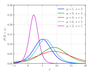
In probability theory, a log-normal (or lognormal) distribution is a continuous probability distribution of a random variable whose logarithm is normally distributed. Thus, if the random variable X is log-normally distributed, then Y = ln(X) has a normal distribution. Equivalently, if Y has a normal distribution, then the exponential function of Y, X = exp(Y), has a log-normal distribution. A random variable which is log-normally distributed takes only positive real values. It is a convenient and useful model for measurements in exact and engineering sciences, as well as medicine, economics and other topics (e.g., energies, concentrations, lengths, prices of financial instruments, and other metrics).

<span class="mw-page-title-main">Weibull distribution</span> Continuous probability distribution

In probability theory and statistics, the Weibull distribution is a continuous probability distribution. It models a broad range of random variables, largely in the nature of a time to failure or time between events. Examples are maximum one-day rainfalls and the time a user spends on a web page.

<span class="mw-page-title-main">Gamma distribution</span> Probability distribution

In probability theory and statistics, the gamma distribution is a versatile two-parameter family of continuous probability distributions. The exponential distribution, Erlang distribution, and chi-squared distribution are special cases of the gamma distribution. There are two equivalent parameterizations in common use:

  1. With a shape parameter k and a scale parameter θ
  2. With a shape parameter and an inverse scale parameter , called a rate parameter.
<span class="mw-page-title-main">Logistic regression</span> Statistical model for a binary dependent variable

In statistics, the logistic model is a statistical model that models the log-odds of an event as a linear combination of one or more independent variables. In regression analysis, logistic regression is estimating the parameters of a logistic model. Formally, in binary logistic regression there is a single binary dependent variable, coded by an indicator variable, where the two values are labeled "0" and "1", while the independent variables can each be a binary variable or a continuous variable. The corresponding probability of the value labeled "1" can vary between 0 and 1, hence the labeling; the function that converts log-odds to probability is the logistic function, hence the name. The unit of measurement for the log-odds scale is called a logit, from logistic unit, hence the alternative names. See § Background and § Definition for formal mathematics, and § Example for a worked example.

<span class="mw-page-title-main">Gumbel distribution</span> Particular case of the generalized extreme value distribution

In probability theory and statistics, the Gumbel distribution is used to model the distribution of the maximum of a number of samples of various distributions.

<span class="mw-page-title-main">Logistic distribution</span> Continuous probability distribution

In probability theory and statistics, the logistic distribution is a continuous probability distribution. Its cumulative distribution function is the logistic function, which appears in logistic regression and feedforward neural networks. It resembles the normal distribution in shape but has heavier tails. The logistic distribution is a special case of the Tukey lambda distribution.

In statistics, a generalized linear model (GLM) is a flexible generalization of ordinary linear regression. The GLM generalizes linear regression by allowing the linear model to be related to the response variable via a link function and by allowing the magnitude of the variance of each measurement to be a function of its predicted value.

In statistics, the Bhattacharyya distance is a quantity which represents a notion of similarity between two probability distributions. It is closely related to the Bhattacharyya coefficient, which is a measure of the amount of overlap between two statistical samples or populations.

<span class="mw-page-title-main">Stable distribution</span> Distribution of variables which satisfies a stability property under linear combinations

In probability theory, a distribution is said to be stable if a linear combination of two independent random variables with this distribution has the same distribution, up to location and scale parameters. A random variable is said to be stable if its distribution is stable. The stable distribution family is also sometimes referred to as the Lévy alpha-stable distribution, after Paul Lévy, the first mathematician to have studied it.

In probability theory and statistics, the generalized extreme value (GEV) distribution is a family of continuous probability distributions developed within extreme value theory to combine the Gumbel, Fréchet and Weibull families also known as type I, II and III extreme value distributions. By the extreme value theorem the GEV distribution is the only possible limit distribution of properly normalized maxima of a sequence of independent and identically distributed random variables. Note that a limit distribution needs to exist, which requires regularity conditions on the tail of the distribution. Despite this, the GEV distribution is often used as an approximation to model the maxima of long (finite) sequences of random variables.

<span class="mw-page-title-main">Pearson distribution</span> Family of continuous probability distributions

The Pearson distribution is a family of continuous probability distributions. It was first published by Karl Pearson in 1895 and subsequently extended by him in 1901 and 1916 in a series of articles on biostatistics.

<span class="mw-page-title-main">Q–Q plot</span> Plot of the empirical distribution of p-values against the theoretical one

In statistics, a Q–Q plot (quantile–quantile plot) is a probability plot, a graphical method for comparing two probability distributions by plotting their quantiles against each other. A point (x, y) on the plot corresponds to one of the quantiles of the second distribution (y-coordinate) plotted against the same quantile of the first distribution (x-coordinate). This defines a parametric curve where the parameter is the index of the quantile interval.

In statistics, binomial regression is a regression analysis technique in which the response has a binomial distribution: it is the number of successes in a series of independent Bernoulli trials, where each trial has probability of success . In binomial regression, the probability of a success is related to explanatory variables: the corresponding concept in ordinary regression is to relate the mean value of the unobserved response to explanatory variables.

In probability and statistics, a natural exponential family (NEF) is a class of probability distributions that is a special case of an exponential family (EF).

<span class="mw-page-title-main">Quantile function</span> Statistical function that defines the quantiles of a probability distribution

In probability and statistics, the quantile function outputs the value of a random variable such that its probability is less than or equal to an input probability value. Intuitively, the quantile function associates with a range at and below a probability input the likelihood that a random variable is realized in that range for some probability distribution. It is also called the percentile function, percent-point function, inverse cumulative distribution function or inverse distribution function.

<span class="mw-page-title-main">Log-logistic distribution</span> Continuous probability distribution for a non-negative random variable

In probability and statistics, the log-logistic distribution is a continuous probability distribution for a non-negative random variable. It is used in survival analysis as a parametric model for events whose rate increases initially and decreases later, as, for example, mortality rate from cancer following diagnosis or treatment. It has also been used in hydrology to model stream flow and precipitation, in economics as a simple model of the distribution of wealth or income, and in networking to model the transmission times of data considering both the network and the software.

Johnsons <i>S<sub>U</sub></i>-distribution Family of probability distributions

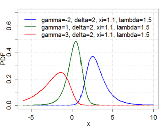
The Johnson's SU-distribution is a four-parameter family of probability distributions first investigated by N. L. Johnson in 1949. Johnson proposed it as a transformation of the normal distribution:

<span class="mw-page-title-main">Metalog distribution</span>

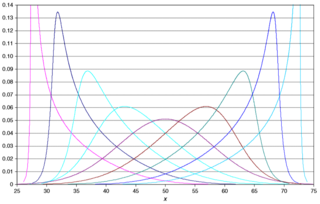
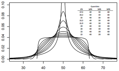
The metalog distribution is a flexible continuous probability distribution designed for ease of use in practice. Together with its transforms, the metalog family of continuous distributions is unique because it embodies all of following properties: virtually unlimited shape flexibility; a choice among unbounded, semi-bounded, and bounded distributions; ease of fitting to data with linear least squares; simple, closed-form quantile function equations that facilitate simulation; a simple, closed-form PDF; and Bayesian updating in closed form in light of new data. Moreover, like a Taylor series, metalog distributions may have any number of terms, depending on the degree of shape flexibility desired and other application needs.

References

  1. Johnson NL, Kotz S, Balakrishnan N. Continuous univariate distributions, Vol 1, Second Edition, John Wiley & Sons, Ltd, 1994, pp. 15–25.
  2. Johnson, N. L. (1949). "Systems of Frequency Curves Generated by Methods of Translation". Biometrika. 36 (1/2): 149–176. doi:10.2307/2332539. JSTOR   2332539. PMID   18132090.
  3. Tadikamalla, Pandu R.; Johnson, Norman L. (1982). "Systems of Frequency Curves Generated by Transformations of Logistic Variables". Biometrika. 69 (2): 461–465. doi:10.1093/biomet/69.2.461. JSTOR   2335422.
  4. 1 2 3 4 5 6 7 Keelin, Thomas W.; Powley, Bradford W. (2011). "Quantile-Parameterized Distributions". Decision Analysis. 8 (3): 206–219. doi:10.1287/deca.1110.0213.
  5. 1 2 Keelin, Thomas W. (2016). "The Metalog Distributions". Decision Analysis. 13 (4): 243–277. doi:10.1287/deca.2016.0338.
  6. 1 2 Faber, Isaac Justin; Paté-Cornell, M. Elisabeth; Lin, Herbert; Shachter, Ross D. (2019). Cyber risk management :AI-generated warnings of threats (Thesis). Stanford University.
  7. Keelin, Thomas W. (2016). "The Metalog Distributions". Decision Analysis. 13 (4). Table 8. doi:10.1287/deca.2016.0338.
  8. Gilchrist, W., 2000. Statistical modelling with quantile functions. CRC Press.
  9. Keelin, Thomas W. (2016). "The Metalog Distributions". Decision Analysis. 13 (4). Section 3, pp. 249–257. doi:10.1287/deca.2016.0338.
  10. 1 2 Keelin, Thomas W. (2016). "The Metalog Distributions". Decision Analysis. 13 (4). Section 4. doi:10.1287/deca.2016.0338.
  11. Powley, B.W. (2013). “Quantile Function Methods For Decision Analysis”. Corollary 12, p 30. PhD Dissertation, Stanford University
  12. Keelin, Thomas W.; Powley, Bradford W. (2011). "Quantile-Parameterized Distributions". Decision Analysis. 8 (3). pp. 208–210. doi:10.1287/deca.1110.0213.
  13. Keelin, Thomas W. (2016). "The Metalog Distributions". Decision Analysis. 13 (4): 253. doi:10.1287/deca.2016.0338.
  14. Hadlock, Christopher C.; Bickel, J. Eric (2017). "Johnson Quantile-Parameterized Distributions". Decision Analysis. 14: 35–64. doi:10.1287/deca.2016.0343.
  15. Hadlock, Christopher C.; Bickel, J. Eric (2019). "The Generalized Johnson Quantile-Parameterized Distribution System". Decision Analysis. 16: 67–85. doi:10.1287/deca.2018.0376. S2CID   159339224.
  16. Keelin, T.W. (2016), Section 6.2.2, pp. 271–274.
  17. Keelin, T.W. (2016), Section 6.1.1, Figure 10, pp 266–267.
  18. Mustafee, N. (18 May 2020). The metalog distributions and extremely accurate sums of lognormals in closed form. Institute of Electrical and Electronics Engineers (IEEE). pp. 3074–3085. ISBN   9781728132839.
  19. Reinhardt, Jason C.; Chen, Xi; Liu, Wenhao; Manchev, Petar; Paté-Cornell, M. Elisabeth (2016). "Asteroid Risk Assessment: A Probabilistic Approach". Risk Analysis. 36 (2): 244–261. Bibcode:2016RiskA..36..244R. doi:10.1111/risa.12453. PMID   26215051. S2CID   23308354.
  20. Wang, Jiali; Neil, Martin; Fenton, Norman (2020). "A Bayesian network approach for cybersecurity risk assessment implementing and extending the FAIR model". Computers & Security. 89: 101659. doi:10.1016/j.cose.2019.101659. S2CID   209099797.
  21. Bratvold, Reidar B.; Mohus, Erlend; Petutschnig, David; Bickel, Eric (2020). "Production Forecasting: Optimistic and Overconfident—Over and over Again". Spe Reservoir Evaluation & Engineering. 23 (3): 0799–0810. doi:10.2118/195914-PA. S2CID   219661316.
  22. Developments in Demographic Forecasting (PDF). The Springer Series on Demographic Methods and Population Analysis. Vol. 49. 2020. pp. 43–62. doi:10.1007/978-3-030-42472-5. hdl:20.500.12657/42565. ISBN   978-3-030-42471-8. S2CID   226615299.