Radial distribution function

calculation of ${\displaystyle g(r)}$

Radial distribution function for the Lennard-Jones model fluid at ${\displaystyle \scriptstyle T^{*}=0.71,\;n^{*}=0.844}$.

In statistical mechanics, the radial distribution function, (or pair correlation function) ${\displaystyle g(r)}$ in a system of particles (atoms, molecules, colloids, etc.), describes how density varies as a function of distance from a reference particle.

If a given particle is taken to be at the origin O, and if ${\displaystyle \rho =N/V}$ is the average number density of particles, then the local time-averaged density at a distance ${\displaystyle r}$ from O is ${\displaystyle \rho g(r)}$. This simplified definition holds for a homogeneous and isotropic system. A more general case will be considered below.

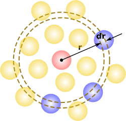
In simplest terms it is a measure of the probability of finding a particle at a distance of ${\displaystyle r}$ away from a given reference particle, relative to that for an ideal gas. The general algorithm involves determining how many particles are within a distance of ${\displaystyle r}$ and ${\displaystyle r+dr}$ away from a particle. This general theme is depicted to the right, where the red particle is our reference particle, and blue particles are those whose centers are within the circular shell, dotted in orange.

The radial distribution function is usually determined by calculating the distance between all particle pairs and binning them into a histogram. The histogram is then normalized with respect to an ideal gas, where particle histograms are completely uncorrelated. For three dimensions, this normalization is the number density of the system ${\displaystyle (\rho )}$ multiplied by the volume of the spherical shell, which symbolically can be expressed as ${\displaystyle \rho \,4\pi r^{2}dr}$.

Given a potential energy function, the radial distribution function can be computed either via computer simulation methods like the Monte Carlo method, or via the Ornstein–Zernike equation, using approximative closure relations like the Percus–Yevick approximation or the Hypernetted Chain Theory. It can also be determined experimentally, by radiation scattering techniques or by direct visualization for large enough (micrometer-sized) particles via traditional or confocal microscopy.

The radial distribution function is of fundamental importance since it can be used, using the Kirkwood–Buff solution theory, to link the microscopic details to macroscopic properties. Moreover, by the reversion of the Kirkwood-Buff theory, it is possible to attain the microscopic details of the radial distribution function from the macroscopic properties. The radial distribution function may also be inverted to predict the potential energy function using the Ornstein-Zernike equation or structure-optimized potential refinement. ^[1]

Definition

Consider a system of ${\displaystyle N}$ particles in a volume ${\displaystyle V}$ (for an average number density ${\displaystyle \rho =N/V}$) and at a temperature ${\displaystyle T}$ (let us also define ${\displaystyle \textstyle \beta ={\frac {1}{kT}}}$; ${\displaystyle k}$ is Boltzmann’s constant). The particle coordinates are ${\displaystyle \mathbf {r} _{i}}$, with ${\displaystyle \textstyle i=1,\,\ldots ,\,N}$. The potential energy due to the interaction between particles is ${\displaystyle \textstyle U_{N}(\mathbf {r} _{1}\,\ldots ,\,\mathbf {r} _{N})}$ and we do not consider the case of an externally applied field.

The appropriate averages are taken in the canonical ensemble ${\displaystyle (N,V,T)}$, with ${\displaystyle \textstyle Z_{N}=\int \cdots \int \mathrm {e} ^{-\beta U_{N}}\mathrm {d} \mathbf {r} _{1}\cdots \mathrm {d} \mathbf {r} _{N}}$ the configurational integral, taken over all possible combinations of particle positions. The probability of an elementary configuration, namely finding particle 1 in ${\displaystyle \textstyle \mathrm {d} \mathbf {r} _{1}}$, particle 2 in ${\displaystyle \textstyle \mathrm {d} \mathbf {r} _{2}}$, etc. is given by

${\displaystyle P^{(N)}(\mathbf {r} _{1},\ldots ,\mathbf {r} _{N})\,\mathrm {d} \mathbf {r} _{1}\cdots \mathrm {d} \mathbf {r} _{N}={\frac {\mathrm {e} ^{-\beta U_{N}}}{Z_{N}}}\,\mathrm {d} \mathbf {r} _{1}\cdots \mathrm {d} \mathbf {r} _{N}\,}$.

(1)

The total number of particles is huge, so that ${\displaystyle P^{(N)}}$ in itself is not very useful. However, one can also obtain the probability of a reduced configuration, where the positions of only ${\displaystyle n<N}$ particles are fixed, in ${\displaystyle \textstyle \mathbf {r} _{1}\,\ldots ,\,\mathbf {r} _{n}}$, with no constraints on the remaining ${\displaystyle N-n}$ particles. To this end, one has to integrate ( 1 ) over the remaining coordinates ${\displaystyle \mathbf {r} _{n+1}\,\ldots ,\,\mathbf {r} _{N}}$:

${\displaystyle P^{(n)}(\mathbf {r} _{1},\ldots ,\mathbf {r} _{n})={\frac {1}{Z_{N}}}\int \cdots \int \mathrm {e} ^{-\beta U_{N}}\,\mathrm {d} ^{3}\mathbf {r} _{n+1}\cdots \mathrm {d} ^{3}\mathbf {r} _{N}\,}$.

If the particles are non-interacting, in the sense that the potential energy of each particle does not depend on any of the other particles, ${\textstyle U_{N}(\mathbf {r} _{1},\dots ,\mathbf {r} _{N})=\sum _{i=1}^{N}U_{1}(\mathbf {r} _{i})}$, then the partition function factorizes, and the probability of an elementary configuration decomposes with independent arguments to a product of single particle probabilities,

${\displaystyle {\begin{aligned}Z_{N}&=\prod _{i=1}^{N}\int \mathrm {d} ^{3}\mathbf {r} _{i}e^{-\beta U_{1}}=Z_{1}^{N}\\P^{(n)}(\mathbf {r} _{1},\dots ,\mathbf {r} _{n})&=P^{(1)}(\mathbf {r} _{1})\cdots P^{(1)}(\mathbf {r} _{n})\end{aligned}}}$

Note how for non-interacting particles the probability is symmetric in its arguments. This is not true in general, and the order in which the positions occupy the argument slots of ${\displaystyle P^{(n)}}$matters. Given a set of positions, the way that the ${\displaystyle N}$ particles can occupy those positions is ${\displaystyle N!}$ The probability that those positions ARE occupied is found by summing over all configurations in which a particle is at each of those locations. This can be done by taking every permutation, ${\displaystyle \pi }$, in the symmetric group on ${\displaystyle N}$ objects, ${\displaystyle S_{N}}$, to write ${\textstyle \sum _{\pi \in S_{N}}P^{(N)}(\mathbf {r} _{\pi (1)},\ldots ,\mathbf {r} _{\pi (N)})}$. For fewer positions, we integrate over extraneous arguments, and include a correction factor to prevent overcounting,

$${\displaystyle {\begin{aligned}\rho ^{(n)}(\mathbf {r} _{1},\ldots ,\mathbf {r} _{n})&={\frac {1}{(N-n)!}}\left(\prod _{i=n+1}^{N}\int \mathrm {d} ^{3}\mathbf {r} _{i}\right)\sum _{\pi \in S_{N}}P^{(N)}(\mathbf {r} _{\pi (1)},\ldots ,\mathbf {r} _{\pi (N)})\\\end{aligned}}}$$

This quantity is called the n-particle density function. For indistinguishable particles, one could permute all the particle positions, ${\displaystyle \forall i,\mathbf {r} _{i}\rightarrow \mathbf {r} _{\pi (i)}}$, without changing the probability of an elementary configuration, ${\displaystyle P(\mathbf {r} _{\pi (1)},\dots ,\mathbf {r} _{\pi (N)})=P(\mathbf {r} _{1},\dots ,\mathbf {r} _{N})}$, so that the n-particle density function reduces to

$${\displaystyle {\begin{aligned}\rho ^{(n)}(\mathbf {r} _{1},\ldots ,\mathbf {r} _{n})&={\frac {N!}{(N-n)!}}P^{(n)}(\mathbf {r} _{1},\ldots ,\mathbf {r} _{n})\end{aligned}}}$$

Integrating the n-particle density gives the permutation factor ${\displaystyle _{N}P_{n}}$, counting the number of ways one can sequentially pick particles to place at the ${\displaystyle n}$ positions out of the total ${\displaystyle N}$ particles. Now let's turn to how we interpret this functions for different values of ${\displaystyle n}$.

For ${\displaystyle n=1}$, we have the one-particle density. For a crystal it is a periodic function with sharp maxima at the lattice sites. For a non-interacting gas, it is independent of the position ${\displaystyle \textstyle \mathbf {r} _{1}}$ and equal to the overall number density, ${\displaystyle \rho }$, of the system. To see this first note that ${\displaystyle U_{N}=\infty }$ in the volume occupied by the gas, and 0 everywhere else. The partition function in this case is

${\displaystyle Z_{N}=\prod _{i=1}^{N}\int \mathrm {d} ^{3}\mathbf {r} _{i}\ 1=V^{N}}$

from which the definition gives the desired result

${\displaystyle {\begin{aligned}\rho ^{(1)}(\mathbf {r} )&={\frac {N!}{(N-1)!}}{\frac {1}{V^{N}}}\prod _{i=2}^{N}\int \mathrm {d} ^{3}\mathbf {r} _{i}1\\&={\frac {N}{V}}\\&=\rho \end{aligned}}}$

In fact, for this special case every n-particle density is independent of coordinates, and can be computed explicitly

$${\displaystyle {\begin{aligned}\rho ^{(n)}(\mathbf {r} _{1},\dots ,\mathbf {r} _{n})&={\frac {N!}{(N-n)!}}{\frac {1}{V^{N}}}\prod _{i=n+1}^{N}\int \mathrm {d} ^{3}\mathbf {r} _{i}1\\&={\frac {N!}{(N-n)!}}{\frac {1}{V^{n}}}\end{aligned}}}$$

For ${\displaystyle N\gg n}$, the non-interacting n-particle density is approximately ${\displaystyle \rho _{\text{non-interacting}}^{(n)}(\mathbf {r} _{1},\dots ,\mathbf {r} _{N})=\left(1-n(n-1)/2N+\cdots \right)\rho ^{n}\approx \rho ^{n}}$. ^[2] With this in hand, the n-point correlation function ${\displaystyle g^{(n)}}$ is defined by factoring out the non-interacting contribution^{[ citation needed ]},

$${\displaystyle \rho ^{(n)}(\mathbf {r} _{1},\ldots ,\,\mathbf {r} _{n})=\rho _{\text{non-interacting}}^{(n)}g^{(n)}(\mathbf {r} _{1}\,\ldots ,\,\mathbf {r} _{n})}$$

Explicitly, this definition reads

$${\displaystyle {\begin{aligned}g^{(n)}(\mathbf {r} _{1},\ldots ,\,\mathbf {r} _{n})&={\frac {V^{N}}{N!}}\left(\prod _{i=n+1}^{N}{\frac {1}{V}}\!\!\int \!\!\mathrm {d} ^{3}\mathbf {r} _{i}\right){\frac {1}{Z_{N}}}\sum _{\pi \in S_{N}}e^{-\beta U(\mathbf {r} _{\pi (1)},\ldots ,\,\mathbf {r} _{\pi (N)})}\end{aligned}}}$$

where it is clear that the n-point correlation function is dimensionless.

Relations involving g(r)

The structure factor

The second-order correlation function ${\displaystyle g^{(2)}(\mathbf {r} _{1},\mathbf {r} _{2})}$ is of special importance, as it is directly related (via a Fourier transform) to the structure factor of the system and can thus be determined experimentally using X-ray diffraction or neutron diffraction. ^[3]

If the system consists of spherically symmetric particles, ${\displaystyle g^{(2)}(\mathbf {r} _{1},\mathbf {r} _{2})}$ depends only on the relative distance between them, ${\displaystyle \mathbf {r} _{12}=\mathbf {r} _{2}-\mathbf {r} _{1}}$. We will drop the sub- and superscript: ${\displaystyle \textstyle g(\mathbf {r} )\equiv g^{(2)}(\mathbf {r} _{12})}$. Taking particle 0 as fixed at the origin of the coordinates, ${\displaystyle \textstyle \rho g(\mathbf {r} )d^{3}r=\mathrm {d} n(\mathbf {r} )}$ is the average number of particles (among the remaining ${\displaystyle N-1}$) to be found in the volume ${\displaystyle \textstyle d^{3}r}$ around the position ${\displaystyle \textstyle \mathbf {r} }$.

We can formally count these particles and take the average via the expression ${\displaystyle \textstyle {\frac {\mathrm {d} n(\mathbf {r} )}{d^{3}r}}=\langle \sum _{i\neq 0}\delta (\mathbf {r} -\mathbf {r} _{i})\rangle }$, with ${\displaystyle \textstyle \langle \cdot \rangle }$ the ensemble average, yielding:

${\displaystyle g(\mathbf {r} )={\frac {1}{\rho }}\langle \sum _{i\neq 0}\delta (\mathbf {r} -\mathbf {r} _{i})\rangle =V{\frac {N-1}{N}}\left\langle \delta (\mathbf {r} -\mathbf {r} _{1})\right\rangle }$

(5)

where the second equality requires the equivalence of particles ${\displaystyle \textstyle 1,\,\ldots ,\,N-1}$. The formula above is useful for relating ${\displaystyle g(\mathbf {r} )}$ to the static structure factor ${\displaystyle S(\mathbf {q} )}$, defined by ${\displaystyle \textstyle S(\mathbf {q} )=\langle \sum _{ij}\mathrm {e} ^{-i\mathbf {q} (\mathbf {r} _{i}-\mathbf {r} _{j})}\rangle /N}$, since we have:

${\displaystyle {\begin{aligned}S(\mathbf {q} )&=1+{\frac {1}{N}}\langle \sum _{i\neq j}\mathrm {e} ^{-i\mathbf {q} (\mathbf {r} _{i}-\mathbf {r} _{j})}\rangle =1+{\frac {1}{N}}\left\langle \int _{V}\mathrm {d} \mathbf {r} \,\mathrm {e} ^{-i\mathbf {q} \mathbf {r} }\sum _{i\neq j}\delta \left[\mathbf {r} -(\mathbf {r} _{i}-\mathbf {r} _{j})\right]\right\rangle \\&=1+{\frac {N(N-1)}{N}}\int _{V}\mathrm {d} \mathbf {r} \,\mathrm {e} ^{-i\mathbf {q} \mathbf {r} }\left\langle \delta (\mathbf {r} -\mathbf {r} _{1})\right\rangle ,\end{aligned}}}$

and thus:

${\displaystyle S(\mathbf {q} )=1+\rho \int _{V}\mathrm {d} \mathbf {r} \,\mathrm {e} ^{-i\mathbf {q} \mathbf {r} }g(\mathbf {r} )}$, proving the Fourier relation alluded to above.

This equation is only valid in the sense of distributions, since ${\displaystyle g(\mathbf {r} )}$ is not normalized: ${\displaystyle \textstyle \lim _{r\rightarrow \infty }g(\mathbf {r} )=1}$, so that ${\displaystyle \textstyle \int _{V}\mathrm {d} \mathbf {r} g(\mathbf {r} )}$ diverges as the volume ${\displaystyle V}$, leading to a Dirac peak at the origin for the structure factor. Since this contribution is inaccessible experimentally we can subtract it from the equation above and redefine the structure factor as a regular function:

${\displaystyle S'(\mathbf {q} )=S(\mathbf {q} )-\rho \delta (\mathbf {q} )=1+\rho \int _{V}\mathrm {d} \mathbf {r} \,\mathrm {e} ^{-i\mathbf {q} \mathbf {r} }[g(\mathbf {r} )-1]}$.

Finally, we rename ${\displaystyle S(\mathbf {q} )\equiv S'(\mathbf {q} )}$ and, if the system is a liquid, we can invoke its isotropy:

${\displaystyle S(q)=1+\rho \int _{V}\mathrm {d} \mathbf {r} \,\mathrm {e} ^{-i\mathbf {q} \mathbf {r} }[g(r)-1]=1+4\pi \rho {\frac {1}{q}}\int \mathrm {d} r\,r\,\mathrm {sin} (qr)[g(r)-1]}$.

(6)

The compressibility equation

Evaluating ( 6 ) in ${\displaystyle q=0}$ and using the relation between the isothermal compressibility ${\displaystyle \textstyle \chi _{T}}$ and the structure factor at the origin yields the compressibility equation:

${\displaystyle \rho kT\chi _{T}=kT\left({\frac {\partial \rho }{\partial p}}\right)=1+\rho \int _{V}\mathrm {d} \mathbf {r} \,[g(r)-1]}$.

(7)

The potential of mean force

It can be shown ^[4] that the radial distribution function is related to the two-particle potential of mean force ${\displaystyle w^{(2)}(r)}$ by:

${\displaystyle g(r)=\exp \left[-{\frac {w^{(2)}(r)}{kT}}\right]}$.

(8)

In the dilute limit, the potential of mean force is the exact pair potential under which the equilibrium point configuration has a given ${\displaystyle g(r)}$.

The energy equation

If the particles interact via identical pairwise potentials: ${\displaystyle \textstyle U_{N}=\sum _{i>j=1}^{N}u(\left|\mathbf {r} _{i}-\mathbf {r} _{j}\right|)}$, the average internal energy per particle is: ^{[5] : Section 2.5}

${\displaystyle {\frac {\left\langle E\right\rangle }{N}}={\frac {3}{2}}kT+{\frac {\left\langle U_{N}\right\rangle }{N}}={\frac {3}{2}}kT+{\frac {\rho }{2}}\int _{V}\mathrm {d} \mathbf {r} \,u(r)g(r,\rho ,T)}$.

(9)

The pressure equation of state

Developing the virial equation yields the pressure equation of state:

${\displaystyle p=\rho kT-{\frac {\rho ^{2}}{6}}\int _{V}\mathrm {d} \mathbf {r} \,rg(r,\rho ,T){\frac {\mathrm {d} u(r)}{\mathrm {d} r}}}$.

(10)

Thermodynamic properties in 3D

The radial distribution function is an important measure because several key thermodynamic properties, such as potential energy and pressure can be calculated from it.

For a 3-D system where particles interact via pairwise potentials, the potential energy of the system can be calculated as follows: ^[6]

${\displaystyle PE={\frac {N}{2}}4\pi \rho \int _{0}^{\infty }r^{2}u(r)g(r)dr}$

Where N is the number of particles in the system, ${\displaystyle \rho }$ is the number density, ${\displaystyle u(r)}$ is the pair potential.

The pressure of the system can also be calculated by relating the 2nd virial coefficient to ${\displaystyle g(r)}$ . The pressure can be calculated as follows: ^[6]

${\displaystyle P=\rho kT-{\frac {2}{3}}\pi \rho ^{2}\int _{0}^{\infty }dr{\frac {du(r)}{dr}}r^{3}g(r)}$.

Note that the results of potential energy and pressure will not be as accurate as directly calculating these properties because of the averaging involved with the calculation of ${\displaystyle g(r)}$.

Approximations

For dilute systems (e.g. gases), the correlations in the positions of the particles that ${\displaystyle g(r)}$ accounts for are only due to the potential ${\displaystyle u(r)}$ engendered by the reference particle, neglecting indirect effects. In the first approximation, it is thus simply given by the Boltzmann distribution law:

${\displaystyle g(r)=\exp \left[-{\frac {u(r)}{kT}}\right]}$.

(11)

If ${\displaystyle u(r)}$ were zero for all ${\displaystyle r}$– i.e., if the particles did not exert any influence on each other, then ${\displaystyle g(r)=1}$ for all ${\displaystyle \mathbf {r} }$ and the mean local density would be equal to the mean density ${\displaystyle \rho }$: the presence of a particle at O would not influence the particle distribution around it and the gas would be ideal. For distances ${\displaystyle r}$ such that ${\displaystyle u(r)}$ is significant, the mean local density will differ from the mean density ${\displaystyle \rho }$, depending on the sign of ${\displaystyle u(r)}$ (higher for negative interaction energy and lower for positive ${\displaystyle u(r)}$).

As the density of the gas increases, the low-density limit becomes less and less accurate since a particle situated in ${\displaystyle \mathbf {r} }$ experiences not only the interaction with the particle in O but also with the other neighbours, themselves influenced by the reference particle. This mediated interaction increases with the density, since there are more neighbours to interact with: it makes physical sense to write a density expansion of ${\displaystyle g(r)}$, which resembles the virial equation:

${\displaystyle g(r)=\exp \left[-{\frac {u(r)}{kT}}\right]y(r)\quad \mathrm {with} \quad y(r)=1+\sum _{n=1}^{\infty }\rho ^{n}y_{n}(r)}$.

(12)

This similarity is not accidental; indeed, substituting ( 12 ) in the relations above for the thermodynamic parameters (Equations 7 , 9 and 10 ) yields the corresponding virial expansions. ^[7] The auxiliary function ${\displaystyle y(r)}$ is known as the cavity distribution function. ^{[5] : Table 4.1} It has been shown that for classical fluids at a fixed density and a fixed positive temperature, the effective pair potential that generates a given ${\displaystyle g(r)}$ under equilibrium is unique up to an additive constant, if it exists. ^[8]

In recent years, some attention has been given to develop pair correlation functions for spatially-discrete data such as lattices or networks. ^[9]

Experimental

One can determine ${\displaystyle g(r)}$ indirectly (via its relation with the structure factor ${\displaystyle S(q)}$) using neutron scattering or x-ray scattering data. The technique can be used at very short length scales (down to the atomic level ^[10] ) but involves significant space and time averaging (over the sample size and the acquisition time, respectively). In this way, the radial distribution function has been determined for a wide variety of systems, ranging from liquid metals ^[11] to charged colloids. ^[12] Going from the experimental ${\displaystyle S(q)}$ to ${\displaystyle g(r)}$ is not straightforward and the analysis can be quite involved. ^[13]

It is also possible to calculate ${\displaystyle g(r)}$ directly by extracting particle positions from traditional or confocal microscopy. ^[14] This technique is limited to particles large enough for optical detection (in the micrometer range), but it has the advantage of being time-resolved so that, aside from the statical information, it also gives access to dynamical parameters (e.g. diffusion constants ^[15] ) and also space-resolved (to the level of the individual particle), allowing it to reveal the morphology and dynamics of local structures in colloidal crystals, ^[16] glasses, ^{[17] [18]} gels, ^{[19] [20]} and hydrodynamic interactions. ^[21]

Direct visualization of a full (distance-dependent and angle-dependent) pair correlation function was achieved by a scanning tunneling microscopy in the case of 2D molecular gases. ^[22]

Higher-order correlation functions

It has been noted that radial distribution functions alone are insufficient to characterize structural information. Distinct point processes may possess identical or practically indistinguishable radial distribution functions, known as the degeneracy problem. ^{[23] [24]} In such cases, higher order correlation functions are needed to further describe the structure.

Higher-order distribution functions ${\displaystyle \textstyle g^{(k)}}$ with ${\displaystyle \textstyle k>2}$ were less studied, since they are generally less important for the thermodynamics of the system; at the same time, they are not accessible by conventional scattering techniques. They can however be measured by coherent X-ray scattering and are interesting insofar as they can reveal local symmetries in disordered systems. ^[25]

See also

• Ornstein–Zernike equation
• Structure Factor

References

1. Shanks, B.; Potoff, J.; Hoepfner, M. (December 5, 2022). "Transferable Force Fields from Experimental Scattering Data with Machine Learning Assisted Structure Refinement". J. Phys. Chem. Lett. 13 (49): 11512–11520. doi:10.1021/acs.jpclett.2c03163. PMID   36469859. S2CID   254274307.
2. Tricomi, F.; Erdélyi, A. (March 1, 1951). "The asymptotic expansion of a ratio of gamma functions". Pacific Journal of Mathematics. 1 (1): 133–142. doi: 10.2140/pjm.1951.1.133 .
3. Dinnebier, R E; Billinge, S J L (March 10, 2008). Powder Diffraction: Theory and Practice (1st ed.). Royal Society of Chemistry. pp.  470–473. doi:10.1039/9781847558237. ISBN   978-1-78262-599-5.
4. Chandler, D. (1987). "7.3". Introduction to Modern Statistical Mechanics. Oxford University Press.
5. Hansen, J. P. and McDonald, I. R. (2005). Theory of Simple Liquids (3rd ed.). Academic Press.
6. Frenkel, Daan; Smit, Berend (2002). Understanding molecular simulation from algorithms to applications (2nd ed.). San Diego: Academic Press. ISBN   978-0122673511.
7. Barker, J.; Henderson, D. (1976). "What is "liquid"? Understanding the states of matter". Reviews of Modern Physics. 48 (4): 587. Bibcode:1976RvMP...48..587B. doi:10.1103/RevModPhys.48.587.
8. Henderson, R. L. (September 9, 1974). "A uniqueness theorem for fluid pair correlation functions". Physics Letters A. 49 (3): 197–198. Bibcode:1974PhLA...49..197H. doi:10.1016/0375-9601(74)90847-0. ISSN   0375-9601.
9. Gavagnin, Enrico (June 4, 2018). "Pair correlation functions for identifying spatial correlation in discrete domains". Physical Review E. 97 (1): 062104. arXiv: 1804.03452 . Bibcode:2018PhRvE..97f2104G. doi:10.1103/PhysRevE.97.062104. PMID   30011502. S2CID   50780864.
10. Yarnell, J.; Katz, M.; Wenzel, R.; Koenig, S. (1973). "Structure Factor and Radial Distribution Function for Liquid Argon at 85 K". Physical Review A. 7 (6): 2130. Bibcode:1973PhRvA...7.2130Y. doi:10.1103/PhysRevA.7.2130.
11. Gingrich, N. S.; Heaton, L. (1961). "Structure of Alkali Metals in the Liquid State". The Journal of Chemical Physics. 34 (3): 873. Bibcode:1961JChPh..34..873G. doi:10.1063/1.1731688.
12. Sirota, E.; Ou-Yang, H.; Sinha, S.; Chaikin, P.; Axe, J.; Fujii, Y. (1989). "Complete phase diagram of a charged colloidal system: A synchro- tron x-ray scattering study". Physical Review Letters. 62 (13): 1524–1527. Bibcode:1989PhRvL..62.1524S. doi:10.1103/PhysRevLett.62.1524. PMID   10039696.
13. Pedersen, J. S. (1997). "Analysis of small-angle scattering data from colloids and polymer solutions: Modeling and least-squares fitting". Advances in Colloid and Interface Science. 70: 171–201. doi:10.1016/S0001-8686(97)00312-6.
14. Crocker, J. C.; Grier, D. G. (1996). "Methods of Digital Video Microscopy for Colloidal Studies". Journal of Colloid and Interface Science. 179 (1): 298–310. Bibcode:1996JCIS..179..298C. doi:10.1006/jcis.1996.0217.
15. Nakroshis, P.; Amoroso, M.; Legere, J.; Smith, C. (2003). "Measuring Boltzmann's constant using video microscopy of Brownian motion". American Journal of Physics. 71 (6): 568. Bibcode:2003AmJPh..71..568N. doi:10.1119/1.1542619.
16. Gasser, U.; Weeks, E. R.; Schofield, A.; Pusey, P. N.; Weitz, D. A. (2001). "Real-Space Imaging of Nucleation and Growth in Colloidal Crystallization". Science. 292 (5515): 258–262. Bibcode:2001Sci...292..258G. doi:10.1126/science.1058457. PMID   11303095. S2CID   6590089.
17. M.I. Ojovan, D.V. Louzguine-Luzgin. Revealing Structural Changes at Glass Transition via Radial Distribution Functions. J. Phys. Chem. B, 124 (15), 3186-3194 (2020) https://doi.org/10.1021/acs.jpcb.0c00214
18. Weeks, E. R.; Crocker, J. C.; Levitt, A. C.; Schofield, A.; Weitz, D. A. (2000). "Three-Dimensional Direct Imaging of Structural Relaxation Near the Colloidal Glass Transition". Science. 287 (5453): 627–631. Bibcode:2000Sci...287..627W. doi:10.1126/science.287.5453.627. PMID   10649991.
19. Cipelletti, L.; Manley, S.; Ball, R. C.; Weitz, D. A. (2000). "Universal Aging Features in the Restructuring of Fractal Colloidal Gels". Physical Review Letters. 84 (10): 2275–2278. Bibcode:2000PhRvL..84.2275C. doi:10.1103/PhysRevLett.84.2275. PMID   11017262.
20. Varadan, P.; Solomon, M. J. (2003). "Direct Visualization of Long-Range Heterogeneous Structure in Dense Colloidal Gels". Langmuir. 19 (3): 509. doi:10.1021/la026303j.
21. Gao, C.; Kulkarni, S. D.; Morris, J. F.; Gilchrist, J. F. (2010). "Direct investigation of anisotropic suspension structure in pressure-driven flow". Physical Review E. 81 (4): 041403. Bibcode:2010PhRvE..81d1403G. doi:10.1103/PhysRevE.81.041403. PMID   20481723.
22. Matvija, Peter; Rozbořil, Filip; Sobotík, Pavel; Ošťádal, Ivan; Kocán, Pavel (2017). "Pair correlation function of a 2D molecular gas directly visualized by scanning tunneling microscopy". The Journal of Physical Chemistry Letters. 8 (17): 4268–4272. doi:10.1021/acs.jpclett.7b01965. PMID   28830146.
23. Stillinger, Frank H.; Torquato, Salvatore (May 28, 2019). "Structural degeneracy in pair distance distributions". The Journal of Chemical Physics. 150 (20): 204125. Bibcode:2019JChPh.150t4125S. doi: 10.1063/1.5096894 . ISSN   0021-9606. PMID   31153177. S2CID   173995240.
24. Wang, Haina; Stillinger, Frank H.; Torquato, Salvatore (September 23, 2020). "Sensitivity of pair statistics on pair potentials in many-body systems". The Journal of Chemical Physics. 153 (12): 124106. Bibcode:2020JChPh.153l4106W. doi: 10.1063/5.0021475 . ISSN   0021-9606. PMID   33003740. S2CID   222169131.
25. Wochner, P.; Gutt, C.; Autenrieth, T.; Demmer, T.; Bugaev, V.; Ortiz, A. D.; Duri, A.; Zontone, F.; Grubel, G.; Dosch, H. (2009). "X-ray cross correlation analysis uncovers hidden local symmetries in disordered matter". Proceedings of the National Academy of Sciences. 106 (28): 11511–4. Bibcode:2009PNAS..10611511W. doi: 10.1073/pnas.0905337106 . PMC   2703671 . PMID   20716512.

• Widom, B. (2002). Statistical Mechanics: A Concise Introduction for Chemists. Cambridge University Press.
• McQuarrie, D. A. (1976). Statistical Mechanics. Harper Collins Publishers.