Lennard-Jones potential

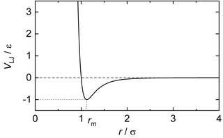
Figure 1. Graph of the Lennard-Jones potential function: Intermolecular potential energy V_LJ as a function of the distance of a pair of particles. The potential minimum is at ${\displaystyle r=r_{\rm {min}}=2^{1/6}\sigma .}$

In computational chemistry, molecular physics, and physical chemistry, the Lennard-Jones potential (also termed the LJ potential or 12-6 potential; named for John Lennard-Jones) is an intermolecular pair potential. Out of all the intermolecular potentials, the Lennard-Jones potential is probably the one that has been the most extensively studied. ^[1] It is considered an archetype model for simple yet realistic intermolecular interactions. The Lennard-Jones potential is often used as a building block in molecular models (a.k.a. force fields) for more complex substances. ^[2] Many studies of an idealized "Lennard-Jones fluid" use the potential to understand the physical nature of the state of fluids. ^[3]

Overview

The Lennard-Jones potential is a simplified model that yet describes the essential features of interactions between simple atoms and molecules: Two interacting particles repel each other at very close distance, attract each other at moderate distance, and eventually stop interacting at infinite distance, as shown in Figure 1. The Lennard-Jones potential is a pair potential, i.e. no three- or multi-body interactions are covered by the potential. ^[2]

The general Lennard-Jones potential combines a repulsive potential, ${\displaystyle 1/r^{n}}$, with an attractive potential, ${\displaystyle -1/r^{m}}$, using empirically determined coefficients ${\displaystyle A_{n}}$ and ${\displaystyle B_{m}}$: ^[2]

$${\displaystyle V_{\text{LJ}}(r)={\frac {A_{n}}{r^{n}}}-{\frac {B_{m}}{r^{m}}}.}$$

In his 1931 review ^[4] Lennard-Jones suggested using ${\displaystyle m=6}$ to match the London dispersion force and ${\displaystyle n=12}$ based matching experimental data. ^[1] Setting ${\displaystyle A_{n}=4\varepsilon \sigma ^{12}}$ and ${\displaystyle B_{m}=4\varepsilon \sigma ^{6}}$ gives the widely used Lennard-Jones 12-6 potential: ^[5]

$${\displaystyle V_{\text{LJ}}(r)=4\varepsilon \left[\left({\frac {\sigma }{r}}\right)^{12}-\left({\frac {\sigma }{r}}\right)^{6}\right],}$$

where r is the distance between two interacting particles, ε is the depth of the potential well, and σ is the distance at which the particle-particle potential energy V is zero. The Lennard-Jones 12-6 potential has its minimum at a distance of ${\displaystyle r=r_{\rm {min}}=2^{1/6}\sigma ,}$ where the potential energy has the value ${\displaystyle V=-\varepsilon .}$

History

In 1924, the year that Lennard-Jones received his PhD from Cambridge University, he published ^{[6] [7]} a series of landmark papers on the pair potentials that would ultimately be named for him. ^[2] In these papers he adjusted the parameters of the potential then using the result in a model of gas viscosity, seeking a set of values consistent with experiment. His initial results suggested a repulsive ${\displaystyle n=13.5}$ and an attractive ${\displaystyle m=3}$.

Before Lennard-Jones, back in 1903, Gustav Mie had worked on effective field theories; Eduard Grüneisen built on Mie work for solids, showing that ${\displaystyle n>m}$ and ${\displaystyle m>3}$ is required for solids. As a result of this work the Lennard-Jones potential is sometimes called the Mie− Grüneisen potential in solid-state physics. ^[2]

In 1930, after the discovery of quantum mechanics, Fritz London showed that theory predicts the long-range attractive force should have ${\displaystyle m=6}$. In 1931, Lennard-Jones applied the this form of the potential to describe many properties of fluids setting the stage for many subsequent studies. ^[1]

Dimensionless (reduced units)

dimensionless (reduced) units

Property	Symbol	Reduced form
Length	${\displaystyle r^{*}}$	${\displaystyle {\frac {r}{\sigma }}}$
Time	${\displaystyle t^{*}}$	${\displaystyle t{\sqrt {\frac {\varepsilon }{m\sigma ^{2}}}}}$
Temperature	${\displaystyle T^{*}}$	${\displaystyle {\frac {k_{B}T}{\varepsilon }}}$
Force	${\displaystyle F^{*}}$	${\displaystyle {\frac {F\sigma }{\varepsilon }}}$
Energy	${\displaystyle U^{*}}$	${\displaystyle {\frac {U}{\varepsilon }}}$
Pressure	${\displaystyle p^{*}}$	${\displaystyle {\frac {p\sigma ^{3}}{\varepsilon }}}$
Density	${\displaystyle \rho ^{*}}$	${\displaystyle \rho \sigma ^{3}}$
Surface tension	${\displaystyle \gamma ^{*}}$	${\displaystyle {\frac {\gamma \sigma ^{2}}{\varepsilon }}}$

Dimensionless reduced units can be defined based on the Lennard-Jones potential parameters, which is convenient for molecular simulations. From a numerical point of view, the advantages of this unit system include computing values which are closer to unity, using simplified equations and being able to easily scale the results. ^{[8] [9]} This reduced units system requires the specification of the size parameter ${\displaystyle \sigma }$ and the energy parameter ${\displaystyle \varepsilon }$ of the Lennard-Jones potential and the mass of the particle ${\displaystyle m}$. All physical properties can be converted straightforwardly taking the respective dimension into account, see table. The reduced units are often abbreviated and indicated by an asterisk.

In general, reduced units can also be built up on other molecular interaction potentials that consist of a length parameter and an energy parameter.

Long-range interactions

Figure 7. Illustrative example of the convergence of a correction scheme to account for the long-range interactions of the Lennard-Jones potential. Therein, ${\displaystyle X}$ indicates an exemplaric observable and ${\displaystyle r_{\mathrm {c} }}$ the applied cut-off radius. The long-range corrected value is indicated as ${\displaystyle X_{\mathrm {corr} }}$ (symbols and line as a guide for the eye); the hypothetical 'true' value as ${\displaystyle X_{\mathrm {true} }}$ (dashed line).

The Lennard-Jones potential, cf. Eq. (1) and Figure 1, has an infinite range. Only under its consideration, the 'true' and 'full' Lennard-Jones potential is examined. For the evaluation of an observable of an ensemble of particles interacting by the Lennard-Jones potential using molecular simulations, the interactions can only be evaluated explicitly up to a certain distance – simply due to the fact that the number of particles will always be finite. The maximum distance applied in a simulation is usually referred to as 'cut-off' radius ${\displaystyle r_{\mathrm {c} }}$ (because the Lennard-Jones potential is radially symmetric). To obtain thermophysical properties (both macroscopic or microscopic) of the 'true' and 'full' Lennard-Jones (LJ) potential, the contribution of the potential beyond the cut-off radius has to be accounted for.

Different corrections schemes have been developed to account for the influence of the long-range interactions in simulations and to sustain a sufficiently good approximation of the 'full' potential. ^{[10] [8]} They are based on simplifying assumptions regarding the structure of the fluid. For simple cases, such as in studies of the equilibrium of homogeneous fluids, simple correction terms yield excellent results. In other cases, such as in studies of inhomogeneous systems with different phases, accounting for the long-range interactions is more tedious. These corrections are usually referred to as 'long-range corrections'. For most properties, simple analytical expressions are known and well established. For a given observable ${\displaystyle X}$, the 'corrected' simulation result ${\displaystyle X_{\mathrm {corr} }}$ is then simply computed from the actually sampled value ${\displaystyle X_{\mathrm {sampled} }}$ and the long-range correction value ${\displaystyle X_{\mathrm {lrc} }}$, e.g. for the internal energy ${\displaystyle U_{\mathrm {corr} }=U_{\mathrm {sampled} }+U_{\mathrm {lrc} }}$. ^[8] The hypothetical true value of the observable of the Lennard-Jones potential at truly infinite cut-off distance (thermodynamic limit) ${\displaystyle X_{\mathrm {true} }}$ can in general only be estimated.

Furthermore, the quality of the long-range correction scheme depends on the cut-off radius. The assumptions made with the correction schemes are usually not justified at (very) short cut-off radii. This is illustrated in the example shown in figure 7. The long-range correction scheme is said to be converged, if the remaining error of the correction scheme is sufficiently small at a given cut-off distance, cf. figure 7.

Extensions and modifications

The Lennard-Jones potential – as an archetype for intermolecular potentials – has been used numerous times as starting point for the development of more elaborate or more generalized intermolecular potentials. Various extensions and modifications of the Lennard-Jones potential have been proposed in the literature; a more extensive list is given in the 'interatomic potential' article. The following list refers only to several example potentials that are directly related to the Lennard-Jones potential and are of both historic importance and still relevant for present research.

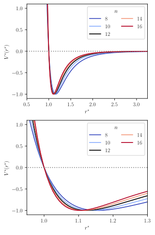
• Mie potential The Mie potential is the generalized version of the Lennard-Jones potential, i.e. the exponents 12 and 6 are introduced as parameters ${\displaystyle \lambda _{\mathrm {rep} }}$ and ${\displaystyle \lambda _{\mathrm {attr} }}$. Especially thermodynamic derivative properties, e.g. the compressibility and the speed of sound, are known to be very sensitive to the steepness of the repulsive part of the intermolecular potential, which can therefore be modeled more sophisticated by the Mie potential. ^[11] The first explicit formulation of the Mie potential is attributed to Eduard Grüneisen. ^{[12] [13]} Hence, the Mie potential was actually proposed before the Lennard-Jones potential. The Mie potential is named after Gustav Mie. ^[14]
• Buckingham potential The Buckingham potential was proposed by Richard Buckingham. The repulsive part of the Lennard-Jones potential is therein replaced by an exponential function and it incorporates an additional parameter.
• Stockmayer potential The Stockmayer potential is named after W.H. Stockmayer. ^[15] The Stockmayer potential is a combination of a Lennard-Jones potential superimposed by a dipole. Hence, Stockmayer particles are not spherically symmetric, but rather have an important orientational structure.
• Two center Lennard-Jones potential The two center Lennard-Jones potential consists of two identical Lennard-Jones interaction sites (same ${\displaystyle \varepsilon }$, ${\displaystyle \sigma }$, ${\displaystyle m}$) that are bonded as a rigid body. It is often abbreviated as 2CLJ. Usually, the elongation (distance between the Lennard-Jones sites) is significantly smaller than the size parameter ${\displaystyle \sigma }$. Hence, the two interaction sites are significantly fused.
• Lennard-Jones truncated & splined potential The Lennard-Jones truncated & splined potential is a rarely used yet useful potential. Similar to the more popular LJTS potential, it is sturdily truncated at a certain 'end' distance ${\displaystyle r_{\mathrm {end} }}$ and no long-range interactions are considered beyond. Opposite to the LJTS potential, which is shifted such that the potential is continuous, the Lennard-Jones truncated & splined potential is made continuous by using an arbitrary but favorable spline function.

Lennard-Jones truncated & shifted (LJTS) potential

Figure 8. Comparison of the vapor–liquid equilibrium of the 'full' Lennard-Jones potential (black) and the 'Lennard-Jones truncated & shifted' potential (blue). The symbols indicate molecular simulation results; the lines indicate results from equations of state.

The Lennard-Jones truncated & shifted (LJTS) potential is an often used alternative to the 'full' Lennard-Jones potential (see Eq. (1)). The 'full' and the 'truncated & shifted' Lennard-Jones potential have to be kept strictly separate. They are simply two different intermolecular potentials yielding different thermophysical properties. The Lennard-Jones truncated & shifted potential is defined as

$${\displaystyle V_{\text{LJTS}}(r)={\begin{cases}V_{\text{LJ}}(r)-V_{\text{LJ}}(r_{\text{end}})&~~~~r\leq r_{\text{end}}\\0&~~~~r>r_{\text{end}},\end{cases}}}$$

with

$${\displaystyle V_{\text{LJ}}(r)=4\varepsilon \left[\left({\frac {\sigma }{r}}\right)^{12}-\left({\frac {\sigma }{r}}\right)^{6}\right].}$$

Hence, the LJTS potential is truncated at ${\displaystyle r_{\mathrm {end} }}$ and shifted by the corresponding energy value ${\displaystyle V_{\mathrm {LJ} }(r_{\mathrm {end} })}$. The latter is applied to avoid a discontinuity jump of the potential at ${\displaystyle r_{\mathrm {end} }}$. For the LJTS potential, no long-range interactions beyond ${\displaystyle r_{\mathrm {end} }}$ are required – neither explicitly nor implicitly. The most frequently used version of the Lennard-Jones truncated & shifted potential is the one with ${\displaystyle r_{\mathrm {end} }=2.5\,\sigma }$.^{[ citation needed ]} Nevertheless, different ${\displaystyle r_{\mathrm {end} }}$ values have been used in the literature. ^{[19] [20] [21] [22]} Each LJTS potential with a given truncation radius ${\displaystyle r_{\mathrm {end} }}$ has to be considered as a potential and accordingly a substance of its own.

The LJTS potential is computationally significantly cheaper than the 'full' Lennard-Jones potential, but still covers the essential physical features of matter (the presence of a critical and a triple point, soft repulsive and attractive interactions, phase equilibria etc.). Therefore, the LJTS potential is used for the testing of new algorithms, simulation methods, and new physical theories. ^{[23] [24] [25]}

Interestingly, for homogeneous systems, the intermolecular forces that are calculated from the LJ and the LJTS potential at a given distance are the same (since ${\displaystyle {\text{d}}V/{\text{d}}r}$ is the same), whereas the potential energy and the pressure are affected by the shifting. Also, the properties of the LJTS substance may furthermore be affected by the chosen simulation algorithm, i.e. MD or MC sampling (this is in general not the case for the 'full' Lennard-Jones potential).

For the LJTS potential with ${\displaystyle r_{\mathrm {end} }=2.5\,\sigma }$, the potential energy shift is approximately 1/60 of the dispersion energy at the potential well: ${\displaystyle V_{\mathrm {LJ} }(r_{\mathrm {end} }=2.5\,\sigma )=-0.0163\,\varepsilon }$. The figure 8 shows the comparison of the vapor–liquid equilibrium of the 'full' Lennard-Jones potential and the 'Lennard-Jones truncated & shifted' potential. The 'full' Lennard-Jones potential results prevail a significantly higher critical temperature and pressure compared to the LJTS potential results, but the critical density is very similar. ^{[26] [27] [21]} The vapor pressure and the enthalpy of vaporization are influenced more strongly by the long-range interactions than the saturated densities. This is due to the fact that the potential is manipulated mainly energetically by the truncation and shifting.

Applications

The Lennard-Jones potential is not only of fundamental importance in computational chemistry and soft-matter physics, but also for the modeling of real substances. The Lennard-Jones potential is used for fundamental studies on the behavior of matter and for elucidating atomistic phenomena. It is also often used for somewhat special use cases, e.g. for studying thermophysical properties of two- or four-dimensional substances ^{[28] [29] [30]} (instead of the classical three spatial directions of our universe).

The Lennard-Jones potential is extensively used for molecular modeling. There are essentially two ways the Lennard-Jones potential can be used for molecular modeling: (1) A real substance atom or molecule is modeled directly by the Lennard-Jones potential, which yields very good results for noble gases and methane, i.e. dispersively interacting spherical particles. In the case of methane, the molecule is assumed to be spherically symmetric and the hydrogen atoms are fused with the carbon atom to a common unit. This simplification can in general also be applied to more complex molecules, but yields usually poor results. (2) A real substance molecule is built of multiple Lennard-Jones interactions sites, which can be connected either by rigid bonds or flexible additional potentials (and eventually also consists of other potential types, e.g. partial charges). Molecular models (often referred to as 'force fields') for practically all molecular and ionic particles can be constructed using this scheme for example for alkanes.

Upon using the first outlined approach, the molecular model has only the two parameters of the Lennard-Jones potential ${\displaystyle \varepsilon }$ and ${\displaystyle \sigma }$ that can be used for the fitting, e.g. ${\displaystyle \varepsilon /k_{\mathrm {B} }=120\,\mathrm {K} }$ and ${\displaystyle \sigma =0.34\,\mathrm {nm} }$ can be used for argon. Evidently, this approach is only a good approximation for spherical and simply dispersively interacting molecules and atoms. The direct use of the Lennard-Jones potential has the great advantage that simulation results and theories for the Lennard-Jones potential can be used directly. Hence, available results for the Lennard-Jones potential and substance can be directly scaled using the appropriate ${\displaystyle \varepsilon }$ and ${\displaystyle \sigma }$ (see reduced units). The Lennard-Jones potential parameters ${\displaystyle \varepsilon }$ and ${\displaystyle \sigma }$ can in general be fitted to any desired real substance property. In soft-matter physics, usually experimental data for the vapor–liquid phase equilibrium or the critical point are used for the parametrization; in solid-state physics, rather the compressibility, heat capacity or lattice constants are employed. ^{[31] [32]}

The second outlined approach of using the Lennard-Jones potential as a building block of elongated and complex molecules is far more sophisticated. Molecular models are thereby tailor-made in a sense that simulation results are only applicable for that particular model. This development approach for molecular force fields is today mainly performed in soft-matter physics and associated fields such as chemical engineering, chemistry, and computational biology. A large number of force fields are based on the Lennard-Jones potential, e.g. the TraPPE force field, ^[33] the OPLS force field, ^[34] and the MolMod force field ^[35] (an overview of molecular force fields is out of the scope of the present article). For the state-of-the-art modeling of solid-state materials, more elaborate multi-body potentials (e.g. EAM potentials ^[36] ) are used.

Lennard-Jones Fluid

A Lennard-Jones fluid or "Lennard-Jonesium" is the name given to an idealized fluid which would result from atoms or molecules interacting exclusively through the Lennard-Jones potential. ^[37] Statistical mechanics ^[38] and computer simulations ^{[9] [10]} can be used to study the Lennard-Jones potential and to obtain thermophysical properties of the 'Lennard-Jones substance'. The Lennard-Jones substance is often referred to as 'Lennard-Jonesium,' ^[37] suggesting that it is viewed as a (fictive) chemical element. ^[16] Moreover, its energy and length parameters can be adjusted to fit many different real substances. Both the Lennard-Jones potential and, accordingly, the Lennard-Jones substance are simplified yet realistic models, such as they accurately capture essential physical principles like the presence of a critical and a triple point, condensation and freezing. Due in part to its mathematical simplicity, the Lennard-Jones potential has been extensively used in studies on matter since the early days of computer simulation. ^{[39] [40] [41] [42]}

Thermophysical properties of the Lennard-Jones substance

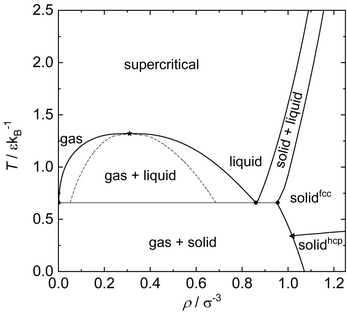
Figure 2. Phase diagram of the Lennard-Jones substance. Correlations and numeric values for the critical point and triple point(s) are taken from Refs. The star indicates the critical point. The circle indicates the vapor–liquid–solid triple point and the triangle indicates the vapor–solid (fcc)–solid (hcp) triple point. The solid lines indicate coexistence lines of two phases. The dashed lines indicate the vapor–liquid spinodal.

Thermophysical properties of the Lennard-Jones substance, ^[37] i.e. particles interacting with the Lennard-Jones potential can be obtained using statistical mechanics. Some properties can be computed analytically, i.e. with machine precision, whereas most properties can only be obtained by performing molecular simulations. ^[9] The latter will in general be superimposed by both statistical and systematic uncertainties. ^{[45] [16] [46] [47]} The virial coefficients can for example be computed directly from the Lennard-potential using algebraic expressions ^[38] and reported data has therefore no uncertainty. Molecular simulation results, e.g. the pressure at a given temperature and density has both statistical and systematic uncertainties. ^{[45] [47]} Molecular simulations of the Lennard-Jones potential can in general be performed using either molecular dynamics (MD) simulations or Monte Carlo (MC) simulation. For MC simulations, the Lennard-Jones potential ${\displaystyle V_{\mathrm {LJ} }(r)}$ is directly used, whereas MD simulations are always based on the derivative of the potential, i.e. the force ${\displaystyle F=\mathrm {d} V/\mathrm {d} r}$. These differences in combination with differences in the treatment of the long-range interactions (see below) can influence computed thermophysical properties. ^{[48] [27]}

Since the Lennard-Jonesium is the archetype for the modeling of simple yet realistic intermolecular interactions, a large number of thermophysical properties were studied and reported in the literature. ^[16] Computer experiment data of the Lennard-Jones potential is presently considered the most accurately known data in classical mechanics computational chemistry. Hence, such data is also mostly used as benchmark for the validation and testing of new algorithms and theories. The Lennard-Jones potential has been constantly used since the early days of molecular simulations. The first results from computer experiments for the Lennard-Jones potential were reported by Rosenbluth and Rosenbluth ^[40] and Wood and Parker ^[39] after molecular simulations on "fast computing machines" became available in 1953. ^[49] Since then many studies reported data of the Lennard-Jones substance; ^[16] approximately 50,000 data points are publicly available. The current state of research of thermophysical properties of the Lennard-Jones substance is summarized in the following. The most comprehensive summary and digital database was given by Stephan et al. ^[16] Presently, no data repository covers and maintains this database (or any other model potential) – the concise data selection stated by the NIST website should be treated with caution regarding referencing ^[50] and coverage (it contains a small fraction of the available data). Most of the data on NIST website provides non-peer-reviewed data generated in-house by NIST.

Figure 2 shows the phase diagram of the Lennard-Jones fluid. Phase equilibria of the Lennard-Jones potential have been studied numerous times and are accordingly known today with good precision. ^{[43] [16] [51]} Figure 2 shows results correlations derived from computer experiment results (hence, lines instead of data points are shown).

The mean intermolecular interaction of a Lennard-Jones particle strongly depends on the thermodynamic state, i.e. temperature and pressure (or density). For solid states, the attractive Lennard-Jones interaction plays a dominant role – especially at low temperatures. For liquid states, no ordered structure is present compared to solid states. The mean potential energy per particle is negative. For gaseous states, attractive interactions of the Lennard-Jones potential play a minor role – since they are far distanced. The main part of the internal energy is stored as kinetic energy for gaseous states. At supercritical states, the attractive Lennard-Jones interaction plays a minor role. With increasing temperature, the mean kinetic energy of the particles increases and exceeds the energy well of the Lennard-Jones potential. Hence, the particles mainly interact by the potentials' soft repulsive interactions and the mean potential energy per particle is accordingly positive.

Overall, due to the large timespan the Lennard-Jones potential has been studied and thermophysical property data has been reported in the literature and computational resources were insufficient for accurate simulations (to modern standards), a noticeable amount of data is known to be dubious. ^[16] Nevertheless, in many studies such data is used as reference. The lack of data repositories and data assessment is a crucial element for future work in the long-going field of Lennard-Jones potential research.

Characteristic points and curves

The most important characteristic points of the Lennard-Jones potential are the critical point and the vapor–liquid–solid triple point. They were studied numerous times in the literature and compiled in Ref. ^[16] The critical point was thereby assessed to be located at

• ${\displaystyle T_{\mathrm {c} }=1.321\pm 0.007\,\varepsilon k_{\mathrm {B} }^{-1}}$
• ${\displaystyle \rho _{\mathrm {c} }=0.316\pm 0.005\,\sigma ^{-3}}$
• ${\displaystyle p_{\mathrm {c} }=0.129\pm 0.005\,\varepsilon \sigma ^{-3}}$

The given uncertainties were calculated from the standard deviation of the critical parameters derived from the most reliable available vapor–liquid equilibrium data sets. ^[16] These uncertainties can be assumed as a lower limit to the accuracy with which the critical point of fluid can be obtained from molecular simulation results.

Figure 3. Characteristic curves of the Lennard-Jones substance. The thick black line indicates the vapor–liquid equilibrium; the star indicates the critical point. The brown line indicates the solid–fluid equilibrium. Other black solid lines and symbols indicate Brown's characteristic curves (see text for details) of the Lennard-Jones substance: lines are results from an equation of state, symbols from molecular simulations and triangles exact data in the ideal gas limit obtained from the virial coefficients. Data taken from.

The triple point is presently assumed to be located at

• ${\displaystyle T_{\mathrm {tr} }=0.69\pm 0.005\,\varepsilon k_{\mathrm {B} }^{-1}}$
• ${\displaystyle \rho _{\mathrm {tr,gas} }=0.0017\pm 0.004\,\sigma ^{-3}}$
• ${\displaystyle \rho _{\mathrm {tr,liq} }=0.845\pm 0.009\,\sigma ^{-3}}$
• ${\displaystyle \rho _{\mathrm {tr,sol} }=0.961\pm 0.007\,\sigma ^{-3}}$
• ${\displaystyle p_{\mathrm {tr} }=0.0012\pm 0.0007\,\varepsilon \sigma ^{-3}}$

The uncertainties represent the scattering of data from different authors. ^[43] The critical point of the Lennard-Jones substance has been studied far more often than the triple point. For both the critical point and the vapor–liquid–solid triple point, several studies reported results out of the above stated ranges. The above stated data is the presently assumed correct and reliable data. Nevertheless, the determinateness of the critical temperature and the triple point temperature is still unsatisfactory.

Evidently, the phase coexistence curves (cf. figure 2) are of fundamental importance to characterize the Lennard-Jones potential. Furthermore, Brown's characteristic curves ^[55] yield an illustrative description of essential features of the Lennard-Jones potential. Brown's characteristic curves are defined as curves on which a certain thermodynamic property of the substance matches that of an ideal gas. For a real fluid, ${\displaystyle Z}$ and its derivatives can match the values of the ideal gas for special ${\displaystyle T}$, ${\displaystyle \rho }$ combinations only as a result of Gibbs' phase rule. The resulting points collectively constitute a characteristic curve. Four main characteristic curves are defined: One 0th-order (named Zeno curve) and three 1st-order curves (named Amagat, Boyle, and Charles curve). The characteristic curve are required to have a negative or zero curvature throughout and a single maximum in a double-logarithmic pressure-temperature diagram. Furthermore, Brown's characteristic curves and the virial coefficients are directly linked in the limit of the ideal gas and are therefore known exactly at ${\displaystyle \rho \rightarrow 0}$. Both computer simulation results and equation of state results have been reported in the literature for the Lennard-Jones potential. ^{[53] [16] [52] [56] [57]}

Points on the Zeno curve Z have a compressibility factor of unity ${\displaystyle Z=p/(\rho T)=1}$. The Zeno curve originates at the Boyle temperature ${\displaystyle T_{\mathrm {B} }=3.417927982\,\varepsilon k_{\mathrm {B} }^{-1}}$, surrounds the critical point, and has a slope of unity in the low temperature limit. ^[52] Points on the Boyle curve B have ${\displaystyle \left.{\frac {\mathrm {d} Z}{\mathrm {d} (1/\rho )}}\right|_{T}=0}$. The Boyle curve originates with the Zeno curve at the Boyle temperature, faintly surrounds the critical point, and ends on the vapor pressure curve. Points on the Charles curve (a.k.a. Joule-Thomson inversion curve) have ${\displaystyle \left.{\frac {\mathrm {d} Z}{\mathrm {d} T}}\right|_{p}=0}$ and more importantly ${\displaystyle \left.{\frac {\mathrm {d} T}{\mathrm {d} p}}\right|_{h}=0}$, i.e. no temperature change upon isenthalpic throttling. It originates at ${\displaystyle T=6.430798418\,\varepsilon k_{\mathrm {B} }^{-1}}$ in the ideal gas limit, crosses the Zeno curve, and terminates on the vapor pressure curve. Points on the Amagat curve A have ${\displaystyle \left.{\frac {\mathrm {d} Z}{\mathrm {d} T}}\right|_{\rho }=0}$. It also starts in the ideal gas limit at ${\displaystyle T=25.15242837\,\varepsilon k_{\mathrm {B} }^{-1}}$, surrounds the critical point and the other three characteristic curves and passes into the solid phase region. A comprehensive discussion of the characteristic curves of the Lennard-Jones potential is given by Stephan and Deiters. ^[52]

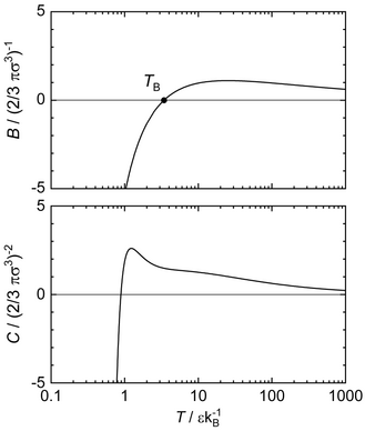
Figure 4. Virial coefficients from the Lennard-Jones potential as a function of the temperature: Second virial coefficient ${\displaystyle B}$ (top) and third virial coefficient ${\displaystyle C}$ (bottom). The circle indicates the Boyle temperature ${\displaystyle T_{\mathrm {B} }}$. Results taken from.

Properties of the Lennard-Jones fluid

Figure 5. Vapor–liquid equilibrium of the Lennard-Jones substance: Vapor pressure (top), saturated densities (middle) and interfacial tension (bottom). Symbols indicate molecular simulation results. Lines indicate results from equation of state (and square gradient theory for the interfacial tension).

Properties of the Lennard-Jones fluid have been studied extensively in the literature due to the outstanding importance of the Lennard-Jones potential in soft-matter physics and related fields. ^[37] About 50 datasets of computer experiment data for the vapor–liquid equilibrium have been published to date. ^[16] Furthermore, more than 35,000 data points at homogeneous fluid states have been published over the years and recently been compiled and assessed for outliers in an open access database. ^[16]

The vapor–liquid equilibrium of the Lennard-Jones substance is presently known with a precision, i.e. mutual agreement of thermodynamically consistent data, of ${\displaystyle \pm 1\%}$ for the vapor pressure, ${\displaystyle \pm 0.2\%}$ for the saturated liquid density, ${\displaystyle \pm 1\%}$ for the saturated vapor density, ${\displaystyle \pm 0.75\%}$ for the enthalpy of vaporization, and ${\displaystyle \pm 4\%}$ for the surface tension. ^[16] This status quo can not be considered satisfactory considering the fact that statistical uncertainties usually reported for single data sets are significantly below the above stated values (even for far more complex molecular force fields).

Both phase equilibrium properties and homogeneous state properties at arbitrary density can in general only be obtained from molecular simulations, whereas virial coefficients can be computed directly from the Lennard-Jones potential. ^[38] Numerical data for the second and third virial coefficient is available in a wide temperature range. ^{[58] [52] [16]} For higher virial coefficients (up to the sixteenth), the number of available data points decreases with increasing number of the virial coefficient. ^{[59] [60]} Also transport properties (viscosity, heat conductivity, and self diffusion coefficient) of the Lennard-Jones fluid have been studied, ^{[61] [62]} but the database is significantly less dense than for homogeneous equilibrium properties like ${\displaystyle pvT}$ – or internal energy data. Moreover, a large number of analytical models (equations of state) have been developed for the description of the Lennard-Jones fluid (see below for details).

Properties of the Lennard-Jones solid

The database and knowledge for the Lennard-Jones solid is significantly poorer than for the fluid phases. It was realized early that the interactions in solid phases should not be approximated to be pair-wise additive – especially for metals. ^{[31] [32]}

Nevertheless, the Lennard-Jones potential is used in solid-state physics due to its simplicity and computational efficiency. Hence, the basic properties of the solid phases and the solid–fluid phase equilibria have been investigated several times, e.g. Refs. ^{[51] [43] [44] [63] [64] [54]}

The Lennard-Jones substance form fcc (face centered cubic), hcp (hexagonal close-packed) and other close-packed polytype lattices – depending on temperature and pressure, cf. figure 2. At low temperature and up to moderate pressure, the hcp lattice is energetically favored and therefore the equilibrium structure. The fcc lattice structure is energetically favored at both high temperature and high pressure and therefore overall the equilibrium structure in a wider state range. The coexistence line between the fcc and hcp phase starts at ${\displaystyle T=0}$ at approximately ${\displaystyle p=878.5\,\varepsilon \sigma ^{-3}}$, passes through a temperature maximum at approximately ${\displaystyle T=0.4\,\varepsilon k_{\mathrm {B} }^{-1}}$, and then ends on the vapor–solid phase boundary at approximately ${\displaystyle T=0.32\,\varepsilon k_{\mathrm {B} }^{-1}}$, which thereby forms a triple point. ^{[63] [43]} Hence, only the fcc solid phase exhibits phase equilibria with the liquid and supercritical phase, cf. figure 2.

The triple point of the two solid phases (fcc and hcp) and the vapor phase is reported to be located at: ^{[63] [43]}

• ${\displaystyle T_{\mathrm {tr} }=0.32\pm 0.001\,\varepsilon k_{\mathrm {B} }^{-1}}$
• ${\displaystyle \rho _{\mathrm {tr,gas} }=..}$ not reported yet
• ${\displaystyle \rho _{\mathrm {tr,fcc} }=1.03859\pm 0.0008\,\sigma ^{-3}}$
• ${\displaystyle \rho _{\mathrm {tr,hcp} }=1.03861\pm 0.0007\,\sigma ^{-3}}$
• ${\displaystyle p_{\mathrm {tr} }=0.96\cdot 10^{-9}\,\varepsilon \sigma ^{-3}}$

Note, that other and significantly differing values have also been reported in the literature. Hence, the database for the fcc-hcp–vapor triple point should be further solidified in the future.

Figure 6. Vapor–liquid equilibria of binary Lennard-Jones mixtures. In all shown cases, component 2 is the more volatile component (enriching in the vapor phase). The units are given in ${\displaystyle \varepsilon }$ and ${\displaystyle \sigma }$ of component 1, which is the same in all four shown mixtures. The temperature is ${\displaystyle T=0.92\,\varepsilon k_{\mathrm {B} }^{-1}}$. Symbols are molecular simulation results and lines are results from an equation of state. Data taken from Ref.

Mixtures of Lennard-Jones substances

Mixtures of Lennard-Jones particles are mostly used as a prototype for the development of theories and methods of solutions, but also to study properties of solutions in general. This dates back to the fundamental work of conformal solution theory of Longuet-Higgins ^[65] and Leland and Rowlinson and co-workers. ^{[66] [67]} Those are today the basis of most theories for mixtures. ^{[68] [69]}

Mixtures of two or more Lennard-Jones components are set up by changing at least one potential interaction parameter (${\displaystyle \varepsilon }$ or ${\displaystyle \sigma }$) of one of the components with respect to the other. For a binary mixture, this yields three types of pair interactions that are all modeled by the Lennard-Jones potential: 1-1, 2-2, and 1-2 interactions. For the cross interactions 1–2, additional assumptions are required for the specification of parameters ${\displaystyle \varepsilon _{\mathrm {12} }}$ or ${\displaystyle \sigma _{\mathrm {12} }}$ from ${\displaystyle \varepsilon _{\mathrm {11} }}$, ${\displaystyle \sigma _{\mathrm {11} }}$ and ${\displaystyle \varepsilon _{\mathrm {22} }}$, ${\displaystyle \sigma _{\mathrm {22} }}$. Various choices (all more or less empirical and not rigorously based on physical arguments) can be used for these so-called combination rules. ^[70] The most widely used ^[70] combination rule is the one of Lorentz and Berthelot ^[71]

$${\displaystyle \sigma _{12}=\eta _{12}{\frac {\sigma _{11}+\sigma _{22}}{2}}}$$

$${\displaystyle \varepsilon _{12}=\xi _{12}{\sqrt {\varepsilon _{11}\varepsilon _{22}}}}$$

The parameter ${\displaystyle \xi _{12}}$ is an additional state-independent interaction parameter for the mixture. The parameter ${\displaystyle \eta _{12}}$ is usually set to unity since the arithmetic mean can be considered physically plausible for the cross-interaction size parameter. The parameter ${\displaystyle \xi _{12}}$ on the other hand is often used to adjust the geometric mean so as to reproduce the phase behavior of the model mixture. For analytical models, e.g. equations of state, the deviation parameter is usually written as ${\displaystyle k_{12}=1-\xi _{12}}$. For ${\displaystyle \xi _{12}>1}$, the cross-interaction dispersion energy and accordingly the attractive force between unlike particles is intensified, and the attractive forces between unlike particles are diminished for ${\displaystyle \xi _{12}<1}$.

For Lennard-Jones mixtures, both fluid and solid phase equilibria can be studied, i.e. vapor–liquid, liquid–liquid, gas–gas, solid–vapor, solid–liquid, and solid–solid. Accordingly, different types of triple points (three-phase equilibria) and critical points can exist as well as different eutectic and azeotropic points. ^{[72] [69]} Binary Lennard-Jones mixtures in the fluid region (various types of equilibria of liquid and gas phases) ^{[26] [73] [74] [75] [76]} have been studied more comprehensively then phase equilibria comprising solid phases. ^{[77] [78] [79] [80] [81]} A large number of different Lennard-Jones mixtures have been studied in the literature. To date, no standard for such has been established. Usually, the binary interaction parameters and the two component parameters are chosen such that a mixture with properties convenient for a given task are obtained. Yet, this often makes comparisons tricky.

For the fluid phase behavior, mixtures exhibit practically ideal behavior (in the sense of Raoult's law) for ${\displaystyle \xi _{12}=1}$. For ${\displaystyle \xi _{12}>1}$ attractive interactions prevail and the mixtures tend to form high-boiling azeotropes, i.e. a lower pressure than pure components' vapor pressures is required to stabilize the vapor–liquid equilibrium. For ${\displaystyle \xi _{12}<1}$ repulsive interactions prevail and mixtures tend to form low-boiling azeotropes, i.e. a higher pressure than pure components' vapor pressures is required to stabilize the vapor–liquid equilibrium since the mean dispersive forces are decreased. Particularly low values of ${\displaystyle \xi _{12}}$ furthermore will result in liquid–liquid miscibility gaps. Also various types of phase equilibria comprising solid phases have been studied in the literature, e.g. by Carol and co-workers. ^{[79] [81] [78] [77]} Also, cases exist where the solid phase boundaries interrupt fluid phase equilibria. However, for phase equilibria that comprise solid phases, the amount of published data is sparse.

Equations of state

A large number of equations of state (EOS) for the Lennard-Jones potential/ substance have been proposed since its characterization and evaluation became available with the first computer simulations. ^[49] Due to the fundamental importance of the Lennard-Jones potential, most currently available molecular-based EOS are built around the Lennard-Jones fluid. They have been comprehensively reviewed by Stephan et al. ^{[3] [52]}

Equations of state for the Lennard-Jones fluid are of particular importance in soft-matter physics and physical chemistry, used as starting point for the development of EOS for complex fluids, e.g. polymers and associating fluids. The monomer units of these models are usually directly adapted from Lennard-Jones EOS as a building block, e.g. the PHC EOS, ^[82] the BACKONE EOS, ^{[83] [84]} and SAFT type EOS. ^{[11] [85] [86] [87]}

More than 30 Lennard-Jones EOS have been proposed in the literature. A comprehensive evaluation ^{[3] [52]} of such EOS showed that several EOS ^{[88] [89] [90] [91]} describe the Lennard-Jones potential with good and similar accuracy, but none of them is outstanding. Three of those EOS show an unacceptable unphysical behavior in some fluid region, e.g. multiple van der Waals loops, while being elsewise reasonably precise. Only the Lennard-Jones EOS of Kolafa and Nezbeda ^[89] was found to be robust and precise for most thermodynamic properties of the Lennard-Jones fluid. ^{[52] [3]} Furthermore, the Lennard-Jones EOS of Johnson et al. ^[92] was found to be less precise for practically all available reference data ^{[16] [3]} than the Kolafa and Nezbeda EOS. ^[89]

See also

• Comparison of force-field implementations
• Embedded atom model
• Force field (chemistry)
• Molecular mechanics
• Morse potential and Morse/Long-range potential
• Virial expansion

References

1. Fischer, Johann; Wendland, Martin (2023-10-01). "On the history of key empirical intermolecular potentials". Fluid Phase Equilibria. 573: 113876. doi:10.1016/j.fluid.2023.113876. ISSN   0378-3812.
2. Schwerdtfeger, Peter; Wales, David J. (2024-04-26). "100 Years of the Lennard-Jones Potential". Journal of Chemical Theory and Computation. doi:10.1021/acs.jctc.4c00135. ISSN   1549-9618.
3. Stephan, Simon; Staubach, Jens; Hasse, Hans (2020). "Review and comparison of equations of state for the Lennard-Jones fluid". Fluid Phase Equilibria. 523: 112772. doi:10.1016/j.fluid.2020.112772. S2CID   224844789.
4. Lennard-Jones, J E (1931-09-01). "Cohesion". Proceedings of the Physical Society. 43 (5): 461–482. Bibcode:1931PPS....43..461L. doi:10.1088/0959-5309/43/5/301. ISSN   0959-5309.
5. Wang, Xipeng; Ramírez-Hinestrosa, Simón; Dobnikar, Jure; Frenkel, Daan (2020). "The Lennard-Jones potential: when (not) to use it". Physical Chemistry Chemical Physics. 22 (19): 10624–10633. doi:10.1039/C9CP05445F. ISSN   1463-9076.
6. Jones, J. E. (1924). "On the determination of molecular fields.—I. From the variation of the viscosity of a gas with temperature". Proceedings of the Royal Society of London. Series A, Containing Papers of a Mathematical and Physical Character. 106 (738): 441–462. Bibcode:1924RSPSA.106..441J. doi: 10.1098/rspa.1924.0081 . ISSN   0950-1207.
7. Jones, J. E. (1924). "On the determination of molecular fields. —II. From the equation of state of a gas". Proceedings of the Royal Society of London. Series A, Containing Papers of a Mathematical and Physical Character. 106 (738): 463–477. Bibcode:1924RSPSA.106..463J. doi: 10.1098/rspa.1924.0082 . ISSN   0950-1207.
8. Allen, Michael P.; Tildesley, Dominic J. (2017-11-23). "Computer Simulation of Liquids". Oxford Scholarship Online. doi:10.1093/oso/9780198803195.001.0001. ISBN   9780198803195.
9. D. C. Rapaport (1 April 2004). The Art of Molecular Dynamics Simulation. Cambridge University Press. ISBN   978-0-521-82568-9.
10. Frenkel, D.; Smit, B. (2002), Understanding Molecular Simulation (Second ed.), San Diego: Academic Press, ISBN   0-12-267351-4
11. Lafitte, Thomas; Apostolakou, Anastasia; Avendaño, Carlos; Galindo, Amparo; Adjiman, Claire S.; Müller, Erich A.; Jackson, George (2013-10-16). "Accurate statistical associating fluid theory for chain molecules formed from Mie segments". The Journal of Chemical Physics. 139 (15): 154504. Bibcode:2013JChPh.139o4504L. doi:10.1063/1.4819786. hdl: 10044/1/12859 . ISSN   0021-9606. PMID   24160524.
12. Grüneisen, Edward (1911). "Das Verhältnis der thermischen Ausdehnung zur spezifischen Wärme fester Elemente". Zeitschrift für Elektrochemie und angewandte physikalische Chemie. 17 (17): 737–739. doi:10.1002/bbpc.191100004. S2CID   178760389.
13. Grüneisen, E. (1912). "Theorie des festen Zustandes einatomiger Elemente". Annalen der Physik (in German). 344 (12): 257–306. Bibcode:1912AnP...344..257G. doi:10.1002/andp.19123441202.
14. Mie, Gustav (1903). "Zur kinetischen Theorie der einatomigen Körper". Annalen der Physik (in German). 316 (8): 657–697. Bibcode:1903AnP...316..657M. doi:10.1002/andp.19033160802.
15. Stockmayer, W. H. (1941-05-01). "Second Virial Coefficients of Polar Gases". The Journal of Chemical Physics. 9 (5): 398–402. Bibcode:1941JChPh...9..398S. doi:10.1063/1.1750922. ISSN   0021-9606.
16. Stephan, Simon; Thol, Monika; Vrabec, Jadran; Hasse, Hans (2019-10-28). "Thermophysical Properties of the Lennard-Jones Fluid: Database and Data Assessment". Journal of Chemical Information and Modeling. 59 (10): 4248–4265. doi:10.1021/acs.jcim.9b00620. ISSN   1549-9596. PMID   31609113. S2CID   204545481.
17. Vrabec, Jadran; Kedia, Gaurav Kumar; Fuchs, Guido; Hasse, Hans (2006-05-10). "Comprehensive study of the vapour–liquid coexistence of the truncated and shifted Lennard–Jones fluid including planar and spherical interface properties". Molecular Physics. 104 (9): 1509–1527. Bibcode:2006MolPh.104.1509V. doi:10.1080/00268970600556774. ISSN   0026-8976. S2CID   96606562.
18. Heier, Michaela; Stephan, Simon; Liu, Jinlu; Chapman, Walter G.; Hasse, Hans; Langenbach, Kai (2018-08-18). "Equation of state for the Lennard-Jones truncated and shifted fluid with a cut-off radius of 2.5 σ based on perturbation theory and its applications to interfacial thermodynamics". Molecular Physics. 116 (15–16): 2083–2094. Bibcode:2018MolPh.116.2083H. doi:10.1080/00268976.2018.1447153. ISSN   0026-8976. S2CID   102956189.
19. Shaul, Katherine R. S.; Schultz, Andrew J.; Kofke, David A. (2010). "The effect of truncation and shift on virial coefficients of Lennard–Jones potentials". Collection of Czechoslovak Chemical Communications. 75 (4): 447–462. doi:10.1135/cccc2009113. ISSN   1212-6950.
20. Shi, Wei; Johnson, J.Karl (2001). "Histogram reweighting and finite-size scaling study of the Lennard–Jones fluids". Fluid Phase Equilibria. 187–188: 171–191. doi:10.1016/S0378-3812(01)00534-9.
21. Dunikov, D. O.; Malyshenko, S. P.; Zhakhovskii, V. V. (2001-10-08). "Corresponding states law and molecular dynamics simulations of the Lennard-Jones fluid". The Journal of Chemical Physics. 115 (14): 6623–6631. Bibcode:2001JChPh.115.6623D. doi:10.1063/1.1396674. ISSN   0021-9606.
22. Lívia B. Pártay, Christoph Ortner, Albert P. Bartók, Chris J. Pickard, and Gábor Csányi "Polytypism in the ground state structure of the Lennard-Jonesium", Physical Chemistry Chemical Physics 19 19369 (2017)
23. Tchipev, Nikola; Seckler, Steffen; Heinen, Matthias; Vrabec, Jadran; Gratl, Fabio; Horsch, Martin; Bernreuther, Martin; Glass, Colin W; Niethammer, Christoph; Hammer, Nicolay; Krischok, Bernd (2019). "TweTriS: Twenty trillion-atom simulation". The International Journal of High Performance Computing Applications. 33 (5): 838–854. doi:10.1177/1094342018819741. ISSN   1094-3420. S2CID   59345875.
24. Stephan, Simon; Liu, Jinlu; Langenbach, Kai; Chapman, Walter G.; Hasse, Hans (2018). "Vapor−Liquid Interface of the Lennard-Jones Truncated and Shifted Fluid: Comparison of Molecular Simulation, Density Gradient Theory, and Density Functional Theory". The Journal of Physical Chemistry C. 122 (43): 24705–24715. doi:10.1021/acs.jpcc.8b06332. ISSN   1932-7447. S2CID   105759822.
25. Kob, Walter; Andersen, Hans C. (1995-05-01). "Testing mode-coupling theory for a supercooled binary Lennard-Jones mixture I: The van Hove correlation function". Physical Review E. 51 (5): 4626–4641. arXiv: cond-mat/9501102 . Bibcode:1995PhRvE..51.4626K. doi:10.1103/PhysRevE.51.4626. PMID   9963176. S2CID   17662741.
26. Stephan, Simon; Hasse, Hans (2020-06-01). "Influence of dispersive long-range interactions on properties of vapour–liquid equilibria and interfaces of binary Lennard-Jones mixtures". Molecular Physics. 118 (9–10): e1699185. Bibcode:2020MolPh.11899185S. doi:10.1080/00268976.2019.1699185. ISSN   0026-8976. S2CID   214174102.
27. Smit, B. (1992), "Phase diagrams of Lennard-Jones fluids" (PDF), Journal of Chemical Physics , 96 (11): 8639–8640, Bibcode:1992JChPh..96.8639S, doi:10.1063/1.462271
28. Smit, B.; Frenkel, D. (1991-04-15). "Vapor–liquid equilibria of the two-dimensional Lennard-Jones fluid(s)". The Journal of Chemical Physics. 94 (8): 5663–5668. Bibcode:1991JChPh..94.5663S. doi:10.1063/1.460477. ISSN   0021-9606. S2CID   1580499.
29. Scalise, Osvaldo H (June 2001). "Type I gas–liquid equilibria of a two-dimensional Lennard–Jones binary mixture". Fluid Phase Equilibria. 182 (1–2): 59–64. doi:10.1016/s0378-3812(01)00380-6. ISSN   0378-3812.
30. Hloucha, M.; Sandler, S. I. (November 1999). "Phase diagram of the four-dimensional Lennard-Jones fluid". The Journal of Chemical Physics. 111 (17): 8043–8047. Bibcode:1999JChPh.111.8043H. doi:10.1063/1.480138. ISSN   0021-9606.
31. Zhen, Shu; Davies, G. J. (1983-08-16). "Calculation of the Lennard-Jonesn–m potential energy parameters for metals". Physica Status Solidi A (in German). 78 (2): 595–605. Bibcode:1983PSSAR..78..595Z. doi:10.1002/pssa.2210780226.
32. Halicioglu, T.; Pound, G. M. (1975-08-16). "Calculation of potential energy parameters form crystalline state properties". Physica Status Solidi A. 30 (2): 619–623. Bibcode:1975PSSAR..30..619H. doi:10.1002/pssa.2210300223.
33. Eggimann, Becky L.; Sunnarborg, Amara J.; Stern, Hudson D.; Bliss, Andrew P.; Siepmann, J. Ilja (2014-01-02). "An online parameter and property database for the TraPPE force field". Molecular Simulation. 40 (1–3): 101–105. doi:10.1080/08927022.2013.842994. ISSN   0892-7022. S2CID   95716947.
34. Jorgensen, William L.; Maxwell, David S.; Tirado-Rives, Julian (January 1996). "Development and Testing of the OPLS All-Atom Force Field on Conformational Energetics and Properties of Organic Liquids". Journal of the American Chemical Society. 118 (45): 11225–11236. doi:10.1021/ja9621760. ISSN   0002-7863.
35. Stephan, Simon; Horsch, Martin T.; Vrabec, Jadran; Hasse, Hans (2019-07-03). "MolMod – an open access database of force fields for molecular simulations of fluids". Molecular Simulation. 45 (10): 806–814. arXiv: 1904.05206 . doi:10.1080/08927022.2019.1601191. ISSN   0892-7022. S2CID   119199372.
36. Mendelev, M. I.; Han, S.; Srolovitz, D. J.; Ackland, G. J.; Sun, D. Y.; Asta, M. (2003). "Development of new interatomic potentials appropriate for crystalline and liquid iron". Philosophical Magazine. 83 (35): 3977–3994. Bibcode:2003PMag...83.3977A. doi:10.1080/14786430310001613264. ISSN   1478-6435. S2CID   4119718.
37. Lenhard, Johannes; Stephan, Simon; Hasse, Hans (February 2024). "A child of prediction. On the History, Ontology, and Computation of the Lennard-Jonesium". Studies in History and Philosophy of Science. 103: 105–113. doi:10.1016/j.shpsa.2023.11.007. PMID   38128443. S2CID   266440296.
38. Hill, Terrell L. (1956). Statistical mechanics: principles and selected applications. New York: Dover Publications. ISBN   0-486-65390-0. OCLC   15163657.
39. Wood, W. W.; Parker, F. R. (1957). "Monte Carlo Equation of State of Molecules Interacting with the Lennard-Jones Potential. I. A Supercritical Isotherm at about Twice the Critical Temperature". The Journal of Chemical Physics. 27 (3): 720–733. Bibcode:1957JChPh..27..720W. doi:10.1063/1.1743822. ISSN   0021-9606.
40. Rosenbluth, Marshall N.; Rosenbluth, Arianna W. (1954). "Further Results on Monte Carlo Equations of State". The Journal of Chemical Physics. 22 (5): 881–884. Bibcode:1954JChPh..22..881R. doi:10.1063/1.1740207. ISSN   0021-9606.
41. Alder, B. J.; Wainwright, T. E. (1959). "Studies in Molecular Dynamics. I. General Method". The Journal of Chemical Physics. 31 (2): 459–466. Bibcode:1959JChPh..31..459A. doi:10.1063/1.1730376. ISSN   0021-9606.
42. Rahman, A. (1964-10-19). "Correlations in the Motion of Atoms in Liquid Argon". Physical Review. 136 (2A): A405–A411. Bibcode:1964PhRv..136..405R. doi:10.1103/PhysRev.136.A405. ISSN   0031-899X.
43. Schultz, Andrew J.; Kofke, David A. (2018-11-28). "Comprehensive high-precision high-accuracy equation of state and coexistence properties for classical Lennard-Jones crystals and low-temperature fluid phases". The Journal of Chemical Physics. 149 (20): 204508. Bibcode:2018JChPh.149t4508S. doi:10.1063/1.5053714. ISSN   0021-9606. PMID   30501268. S2CID   54629914.
44. Schultz, Andrew J.; Kofke, David A. (2020-08-07). "Erratum: "Comprehensive high-precision high-accuracy equation of state and coexistence properties for classical Lennard-Jones crystals and low-temperature fluid phases" [J. Chem. Phys. 149, 204508 (2018)]". The Journal of Chemical Physics. 153 (5): 059901. doi: 10.1063/5.0021283 . ISSN   0021-9606. PMID   32770918.
45. Schappals, Michael; Mecklenfeld, Andreas; Kröger, Leif; Botan, Vitalie; Köster, Andreas; Stephan, Simon; García, Edder J.; Rutkai, Gabor; Raabe, Gabriele; Klein, Peter; Leonhard, Kai (2017-09-12). "Round Robin Study: Molecular Simulation of Thermodynamic Properties from Models with Internal Degrees of Freedom". Journal of Chemical Theory and Computation. 13 (9): 4270–4280. doi:10.1021/acs.jctc.7b00489. ISSN   1549-9618. PMID   28738147.
46. Loeffler, Hannes H.; Bosisio, Stefano; Duarte Ramos Matos, Guilherme; Suh, Donghyuk; Roux, Benoit; Mobley, David L.; Michel, Julien (2018-11-13). "Reproducibility of Free Energy Calculations across Different Molecular Simulation Software Packages". Journal of Chemical Theory and Computation. 14 (11): 5567–5582. doi:10.1021/acs.jctc.8b00544. hdl: 20.500.11820/52d85d71-d3df-468b-8f88-9c52e83da1f1 . ISSN   1549-9618. PMID   30289712. S2CID   52923832.
47. Lenhard, Johannes; Küster, Uwe (2019). "Reproducibility and the Concept of Numerical Solution". Minds and Machines. 29 (1): 19–36. doi:10.1007/s11023-019-09492-9. ISSN   0924-6495. S2CID   59159685.
48. Shi, Wei; Johnson, J. Karl (2001-09-15). "Histogram reweighting and finite-size scaling study of the Lennard–Jones fluids". Fluid Phase Equilibria. 187–188: 171–191. doi:10.1016/S0378-3812(01)00534-9. ISSN   0378-3812.
49. Metropolis, Nicholas; Rosenbluth, Arianna W.; Rosenbluth, Marshall N.; Teller, Augusta H.; Teller, Edward (1953). "Equation of State Calculations by Fast Computing Machines". The Journal of Chemical Physics. 21 (6): 1087–1092. Bibcode:1953JChPh..21.1087M. doi:10.1063/1.1699114. ISSN   0021-9606. OSTI   4390578. S2CID   1046577.
50. Stephan, Simon; Thol, Monika; Vrabec, Jadran; Hasse, Hans (2019-10-28). "Thermophysical Properties of the Lennard-Jones Fluid: Database and Data Assessment". Journal of Chemical Information and Modeling. 59 (10): 4248–4265. doi:10.1021/acs.jcim.9b00620. ISSN   1549-9596. PMID   31609113. S2CID   204545481.
51. Köster, Andreas; Mausbach, Peter; Vrabec, Jadran (2017-10-10). "Premelting, solid–fluid equilibria, and thermodynamic properties in the high density region based on the Lennard-Jones potential". The Journal of Chemical Physics. 147 (14): 144502. Bibcode:2017JChPh.147n4502K. doi:10.1063/1.4990667. ISSN   0021-9606. PMID   29031254.
52. Stephan, Simon; Deiters, Ulrich K. (2020-08-20). "Characteristic Curves of the Lennard-Jones Fluid". International Journal of Thermophysics. 41 (10): 147. Bibcode:2020IJT....41..147S. doi:10.1007/s10765-020-02721-9. ISSN   1572-9567. PMC   7441092 . PMID   32863513.
53. Deiters, Ulrich K.; Neumaier, Arnold (2016-08-11). "Computer Simulation of the Characteristic Curves of Pure Fluids". Journal of Chemical & Engineering Data. 61 (8): 2720–2728. doi:10.1021/acs.jced.6b00133. ISSN   0021-9568.
54. Agrawal, Rupal; Kofke, David A. (1995). "Thermodynamic and structural properties of model systems at solid–fluid coexistence: II. Melting and sublimation of the Lennard-Jones system". Molecular Physics. 85 (1): 43–59. doi:10.1080/00268979500100921. ISSN   0026-8976.
55. Brown, E.H. (1960). "On the thermodynamic properties of fluids". Bulletin de l'Institut International du Froid. Annexe 1960-1: 169–178.
56. Apfelbaum, E. M.; Vorob’ev, V. S. (2020-06-18). "The Line of the Unit Compressibility Factor (Zeno-Line) for Crystal States". The Journal of Physical Chemistry B. 124 (24): 5021–5027. doi:10.1021/acs.jpcb.0c02749. ISSN   1520-6106. PMID   32437611. S2CID   218835048.
57. Apfelbaum, E. M.; Vorob’ev, V. S.; Martynov, G. A. (2008). "Regarding the Theory of the Zeno Line". The Journal of Physical Chemistry A. 112 (26): 6042–6044. Bibcode:2008JPCA..112.6042A. doi:10.1021/jp802999z. ISSN   1089-5639. PMID   18543889.
58. Nicolas, J.J.; Gubbins, K.E.; Streett, W.B.; Tildesley, D.J. (1979). "Equation of state for the Lennard-Jones fluid". Molecular Physics. 37 (5): 1429–1454. Bibcode:1979MolPh..37.1429N. doi:10.1080/00268977900101051. ISSN   0026-8976.
59. Feng, Chao; Schultz, Andrew J.; Chaudhary, Vipin; Kofke, David A. (2015-07-28). "Eighth to sixteenth virial coefficients of the Lennard-Jones model". The Journal of Chemical Physics. 143 (4): 044504. Bibcode:2015JChPh.143d4504F. doi: 10.1063/1.4927339 . ISSN   0021-9606. PMID   26233142.
60. Schultz, Andrew J.; Kofke, David A. (2009-11-10). "Sixth, seventh and eighth virial coefficients of the Lennard-Jones model". Molecular Physics. 107 (21): 2309–2318. Bibcode:2009MolPh.107.2309S. doi:10.1080/00268970903267053. ISSN   0026-8976. S2CID   94811614.
61. Bell, Ian H.; Messerly, Richard; Thol, Monika; Costigliola, Lorenzo; Dyre, Jeppe C. (2019-07-25). "Modified Entropy Scaling of the Transport Properties of the Lennard-Jones Fluid". The Journal of Physical Chemistry B. 123 (29): 6345–6363. doi:10.1021/acs.jpcb.9b05808. ISSN   1520-6106. PMC   7147083 . PMID   31241958.
62. Lautenschlaeger, Martin P.; Hasse, Hans (2019). "Transport properties of the Lennard-Jones truncated and shifted fluid from non-equilibrium molecular dynamics simulations". Fluid Phase Equilibria. 482: 38–47. doi:10.1016/j.fluid.2018.10.019. S2CID   106113718.
63. Travesset, Alex (2014-10-28). "Phase diagram of power law and Lennard-Jones systems: Crystal phases". The Journal of Chemical Physics. 141 (16): 164501. Bibcode:2014JChPh.141p4501T. doi:10.1063/1.4898371. ISSN   0021-9606. PMID   25362319.
64. Hansen, Jean-Pierre; Verlet, Loup (1969-08-05). "Phase Transitions of the Lennard-Jones System". Physical Review. 184 (1): 151–161. Bibcode:1969PhRv..184..151H. doi:10.1103/PhysRev.184.151. ISSN   0031-899X.
65. Longuet-Higgins, H.C. (1951-02-07). "The statistical thermodynamics of multicomponent systems". Proceedings of the Royal Society of London. Series A. Mathematical and Physical Sciences. 205 (1081): 247–269. Bibcode:1951RSPSA.205..247L. doi:10.1098/rspa.1951.0028. ISSN   0080-4630. S2CID   202575459.
66. Leland, T. W.; Rowlinson, J. S.; Sather, G. A. (1968). "Statistical thermodynamics of mixtures of molecules of different sizes". Transactions of the Faraday Society. 64: 1447. doi:10.1039/tf9686401447. ISSN   0014-7672.
67. Mansoori, G. Ali; Leland, Thomas W. (1972). "Statistical thermodynamics of mixtures. A new version for the theory of conformal solution". Journal of the Chemical Society, Faraday Transactions 2. 68: 320. doi:10.1039/f29726800320. ISSN   0300-9238.
68. Rowlinson, J.S.; Swinton, F.L. (1982). Liquids and liquid mixtures (Third ed.). London: Butterworth.
69. Deiters, Ulrich K.; Kraska, Thomas (2012). High-pressure fluid phase equilibria: phenomenology and computation (1st ed.). Amsterdam: Elsevier. ISBN   978-0-444-56354-5. OCLC   787847134.
70. Schnabel, Thorsten; Vrabec, Jadran; Hasse, Hans (2007). "Unlike Lennard–Jones parameters for vapor–liquid equilibria". Journal of Molecular Liquids. 135 (1–3): 170–178. arXiv: 0904.4436 . doi:10.1016/j.molliq.2006.12.024. S2CID   16111477.
71. Lorentz, H. A. (1881). "Ueber die Anwendung des Satzes vom Virial in der kinetischen Theorie der Gase". Annalen der Physik (in German). 248 (1): 127–136. Bibcode:1881AnP...248..127L. doi:10.1002/andp.18812480110.
72. van Konynenburg, P.H.; Scott, R.L. (1980-12-18). "Critical lines and phase equilibria in binary van der Waals mixtures". Philosophical Transactions of the Royal Society of London. Series A, Mathematical and Physical Sciences. 298 (1442): 495–540. Bibcode:1980RSPTA.298..495K. doi:10.1098/rsta.1980.0266. ISSN   0080-4614. S2CID   122538015.
73. Potoff, Jeffrey J.; Panagiotopoulos, Athanassios Z. (1998-12-22). "Critical point and phase behavior of the pure fluid and a Lennard-Jones mixture". The Journal of Chemical Physics. 109 (24): 10914–10920. Bibcode:1998JChPh.10910914P. doi:10.1063/1.477787. ISSN   0021-9606.
74. Protsenko, Sergey P.; Baidakov, Vladimir G. (2016). "Binary Lennard-Jones mixtures with highly asymmetric interactions of the components. 1. Effect of the energy parameters on phase equilibria and properties of liquid–gas interfaces". Fluid Phase Equilibria. 429: 242–253. doi:10.1016/j.fluid.2016.09.009.
75. Protsenko, Sergey P.; Baidakov, Vladimir G.; Bryukhanov, Vasiliy M. (2016). "Binary Lennard-Jones mixtures with highly asymmetric interactions of the components. 2. Effect of the particle size on phase equilibria and properties of liquid–gas interfaces". Fluid Phase Equilibria. 430: 67–74. doi:10.1016/j.fluid.2016.09.022.
76. Stephan, Simon; Hasse, Hans (2020-01-23). "Molecular interactions at vapor–liquid interfaces: Binary mixtures of simple fluids". Physical Review E. 101 (1): 012802. Bibcode:2020PhRvE.101a2802S. doi:10.1103/PhysRevE.101.012802. ISSN   2470-0045. PMID   32069593. S2CID   211192904.
77. Lamm, Monica H.; Hall, Carol K. (2002). "Equilibria between solid, liquid, and vapor phases in binary Lennard–Jones mixtures". Fluid Phase Equilibria. 194–197: 197–206. doi:10.1016/S0378-3812(01)00650-1.
78. Lamm, Monica H.; Hall, Carol K. (2001). "Monte Carlo simulations of complete phase diagrams for binary Lennard–Jones mixtures". Fluid Phase Equilibria. 182 (1–2): 37–46. doi:10.1016/S0378-3812(01)00378-8.
79. Hitchcock, Monica R.; Hall, Carol K. (1999-06-15). "Solid–liquid phase equilibrium for binary Lennard-Jones mixtures". The Journal of Chemical Physics. 110 (23): 11433–11444. Bibcode:1999JChPh.11011433H. doi:10.1063/1.479084. ISSN   0021-9606.
80. Jungblut, Swetlana; Dellago, Christoph (2011-03-14). "Crystallization of a binary Lennard-Jones mixture". The Journal of Chemical Physics. 134 (10): 104501. Bibcode:2011JChPh.134j4501J. doi:10.1063/1.3556664. ISSN   0021-9606. PMID   21405169.
81. Lamm, Monica H.; Hall, Carol K. (2004). "Effect of pressure on the complete phase behavior of binary mixtures". AIChE Journal. 50 (1): 215–225. Bibcode:2004AIChE..50..215L. doi: 10.1002/aic.10020 . ISSN   0001-1541.
82. Cotterman, R. L.; Prausnitz, J. M. (1986). "Molecular thermodynamics for fluids at low and high densities. Part II: Phase equilibria for mixtures containing components with large differences in molecular size or potential energy". AIChE Journal. 32 (11): 1799–1812. Bibcode:1986AIChE..32.1799C. doi:10.1002/aic.690321105. ISSN   0001-1541. S2CID   96417239.
83. Müller, Andreas; Winkelmann, Jochen; Fischer, Johann (1996). "Backone family of equations of state: 1. Nonpolar and polar pure fluids". AIChE Journal. 42 (4): 1116–1126. Bibcode:1996AIChE..42.1116M. doi:10.1002/aic.690420423. ISSN   0001-1541.
84. Weingerl, Ulrike; Wendland, Martin; Fischer, Johann; Müller, Andreas; Winkelmann, Jochen (2001). "Backone family of equations of state: 2. Nonpolar and polar fluid mixtures". AIChE Journal. 47 (3): 705–717. Bibcode:2001AIChE..47..705W. doi:10.1002/aic.690470317.
85. Blas, F.J.; Vega, L.F. (1997). "Thermodynamic behaviour of homonuclear and heteronuclear Lennard-Jones chains with association sites from simulation and theory". Molecular Physics. 92 (1): 135–150. Bibcode:1997MolPh..92..135F. doi:10.1080/002689797170707. ISSN   0026-8976.
86. Kraska, Thomas; Gubbins, Keith E. (1996). "Phase Equilibria Calculations with a Modified SAFT Equation of State. 1. Pure Alkanes, Alkanols, and Water". Industrial & Engineering Chemistry Research. 35 (12): 4727–4737. doi:10.1021/ie9602320. ISSN   0888-5885.
87. Ghonasgi, D.; Chapman, Walter G. (1994). "Prediction of the properties of model polymer solutions and blends". AIChE Journal. 40 (5): 878–887. Bibcode:1994AIChE..40..878G. doi:10.1002/aic.690400514. ISSN   0001-1541.
88. Mecke, M.; Müller, A.; Winkelmann, J.; Vrabec, J.; Fischer, J.; Span, R.; Wagner, W. (1996-03-01). "An accurate Van der Waals-type equation of state for the Lennard-Jones fluid". International Journal of Thermophysics. 17 (2): 391–404. Bibcode:1996IJT....17..391M. doi:10.1007/BF01443399. ISSN   1572-9567. S2CID   123304062.
89. Kolafa, Jiří; Nezbeda, Ivo (1994). "The Lennard-Jones fluid: an accurate analytic and theoretically-based equation of state". Fluid Phase Equilibria. 100: 1–34. doi:10.1016/0378-3812(94)80001-4.
90. Thol, Monika; Rutkai, Gabor; Köster, Andreas; Lustig, Rolf; Span, Roland; Vrabec, Jadran (2016). "Equation of State for the Lennard-Jones Fluid". Journal of Physical and Chemical Reference Data. 45 (2): 023101. Bibcode:2016JPCRD..45b3101T. doi:10.1063/1.4945000. ISSN   0047-2689.
91. Gottschalk, Matthias (2019-12-01). "An EOS for the Lennard-Jones fluid: A virial expansion approach". AIP Advances. 9 (12): 125206. Bibcode:2019AIPA....9l5206G. doi: 10.1063/1.5119761 . ISSN   2158-3226.
92. Johnson, J. Karl; Zollweg, John A.; Gubbins, Keith E. (1993-02-20). "The Lennard-Jones equation of state revisited". Molecular Physics. 78 (3): 591–618. Bibcode:1993MolPh..78..591J. doi:10.1080/00268979300100411. ISSN   0026-8976.

External links

• Lennard-Jones model on SklogWiki.