Radon transform

Last updated
Radon transform. Maps f on the (x, y)-domain to Rf on the (a, s)-domain. Radon transform.png
Radon transform. Maps f on the (x, y)-domain to Rf on the (α, s)-domain.

In mathematics, the Radon transform is the integral transform which takes a function f defined on the plane to a function Rf defined on the (two-dimensional) space of lines in the plane, whose value at a particular line is equal to the line integral of the function over that line. The transform was introduced in 1917 by Johann Radon, [1] who also provided a formula for the inverse transform. Radon further included formulas for the transform in three dimensions, in which the integral is taken over planes (integrating over lines is known as the X-ray transform). It was later generalized to higher-dimensional Euclidean spaces and more broadly in the context of integral geometry. The complex analogue of the Radon transform is known as the Penrose transform. The Radon transform is widely applicable to tomography, the creation of an image from the projection data associated with cross-sectional scans of an object.

Contents

Explanation

Radon transform of the indicator function of two squares shown in the image below. Lighter regions indicate larger function values. Black indicates zero. Sinogram - Two Square Indicator Phantom.svg
Radon transform of the indicator function of two squares shown in the image below. Lighter regions indicate larger function values. Black indicates zero.
Original function is equal to one on the white region and zero on the dark region. Sinogram Source - Two Squares Phantom.svg
Original function is equal to one on the white region and zero on the dark region.

If a function represents an unknown density, then the Radon transform represents the projection data obtained as the output of a tomographic scan. Hence the inverse of the Radon transform can be used to reconstruct the original density from the projection data, and thus it forms the mathematical underpinning for tomographic reconstruction, also known as iterative reconstruction.

The Radon transform data is often called a sinogram because the Radon transform of an off-center point source is a sinusoid. Consequently, the Radon transform of a number of small objects appears graphically as a number of blurred sine waves with different amplitudes and phases.

The Radon transform is useful in computed axial tomography (CAT scan), barcode scanners, electron microscopy of macromolecular assemblies like viruses and protein complexes, reflection seismology and in the solution of hyperbolic partial differential equations.

Horizontal projections through the shape result in an accumulated signal (middle bar). The sinogram on the right is generated by collecting many such projections as the shape rotates. Here, color is used to highlight which object is producing which part of the signal. Note how straight features, when aligned with the projection direction, result in stronger signals. Radon transform sinogram.gif
Horizontal projections through the shape result in an accumulated signal (middle bar). The sinogram on the right is generated by collecting many such projections as the shape rotates. Here, color is used to highlight which object is producing which part of the signal. Note how straight features, when aligned with the projection direction, result in stronger signals.
Example of reconstruction via the Radon transform using observations from different angles. The applied inversion to the projection data then reconstructs the slice image. Radon transform example.jpg
Example of reconstruction via the Radon transform using observations from different angles. The applied inversion to the projection data then reconstructs the slice image.

Definition

Let be a function that satisfies the three regularity conditions: [3]

  1. is continuous;
  2. the double integral , extending over the whole plane, converges;
  3. for any arbitrary point on the plane it holds that


The Radon transform, , is a function defined on the space of straight lines by the line integral along each such line as:

Concretely, the parametrization of any straight line with respect to arc length can always be written:

where is the distance of from the origin and is the angle the normal vector to makes with the -axis. It follows that the quantities can be considered as coordinates on the space of all lines in , and the Radon transform can be expressed in these coordinates by:

More generally, in the -dimensional Euclidean space , the Radon transform of a function satisfying the regularity conditions is a function on the space of all hyperplanes in . It is defined by:

Shepp logan radon.png
Radon transform
Shepp logan iradon.png
Inverse Radon transform

where the integral is taken with respect to the natural hypersurface measure, (generalizing the term from the -dimensional case). Observe that any element of is characterized as the solution locus of an equation , where is a unit vector and . Thus the -dimensional Radon transform may be rewritten as a function on via:

It is also possible to generalize the Radon transform still further by integrating instead over -dimensional affine subspaces of . The X-ray transform is the most widely used special case of this construction, and is obtained by integrating over straight lines.

Relationship with the Fourier transform

Computing the 2-dimensional Radon transform in terms of two Fourier transforms. Radon transform via Fourier transform.png
Computing the 2-dimensional Radon transform in terms of two Fourier transforms.

The Radon transform is closely related to the Fourier transform. We define the univariate Fourier transform here as:

For a function of a -vector , the univariate Fourier transform is:

For convenience, denote . The Fourier slice theorem then states:

where Thus the two-dimensional Fourier transform of the initial function along a line at the inclination angle is the one variable Fourier transform of the Radon transform (acquired at angle ) of that function. This fact can be used to compute both the Radon transform and its inverse. The result can be generalized into n dimensions:

Dual transform

The dual Radon transform is a kind of adjoint to the Radon transform. Beginning with a function g on the space , the dual Radon transform is the function on Rn defined by:

The integral here is taken over the set of all hyperplanes incident with the point , and the measure is the unique probability measure on the set invariant under rotations about the point . Concretely, for the two-dimensional Radon transform, the dual transform is given by:

In the context of image processing, the dual transform is commonly called back-projection [4] as it takes a function defined on each line in the plane and 'smears' or projects it back over the line to produce an image.

Intertwining property

Let denote the Laplacian on defined by:

This is a natural rotationally invariant second-order differential operator. On , the "radial" second derivative is also rotationally invariant. The Radon transform and its dual are intertwining operators for these two differential operators in the sense that: [5]

In analysing the solutions to the wave equation in multiple spatial dimensions, the intertwining property leads to the translational representation of Lax and Philips. [6] In imaging [7] and numerical analysis [8] this is exploited to reduce multi-dimensional problems into single-dimensional ones, as a dimensional splitting method.

Reconstruction approaches

The process of reconstruction produces the image (or function in the previous section) from its projection data. Reconstruction is an inverse problem.

Radon inversion formula

In the two-dimensional case, the most commonly used analytical formula to recover from its Radon transform is the Filtered Back-projection Formula or Radon Inversion Formula [9] :

where is such that . [9] The convolution kernel is referred to as Ramp filter in some literature.

Ill-posedness

Intuitively, in the filtered back-projection formula, by analogy with differentiation, for which , we see that the filter performs an operation similar to a derivative. Roughly speaking, then, the filter makes objects more singular. A quantitive statement of the ill-posedness of Radon inversion goes as follows:

where is the previously defined adjoint to the Radon Transform. Thus for , we have:

The complex exponential is thus an eigenfunction of with eigenvalue . Thus the singular values of are . Since these singular values tend to , is unbounded. [9]

Iterative reconstruction methods

Compared with the Filtered Back-projection method, iterative reconstruction costs large computation time, limiting its practical use. However, due to the ill-posedness of Radon Inversion, the Filtered Back-projection method may be infeasible in the presence of discontinuity or noise. Iterative reconstruction methods (e.g. iterative Sparse Asymptotic Minimum Variance [10] ) could provide metal artefact reduction, noise and dose reduction for the reconstructed result that attract much research interest around the world.

Inversion formulas

Explicit and computationally efficient inversion formulas for the Radon transform and its dual are available. The Radon transform in dimensions can be inverted by the formula: [11]

where , and the power of the Laplacian is defined as a pseudo-differential operator if necessary by the Fourier transform:

For computational purposes, the power of the Laplacian is commuted with the dual transform to give: [12]

where is the Hilbert transform with respect to the s variable. In two dimensions, the operator appears in image processing as a ramp filter. [13] One can prove directly from the Fourier slice theorem and change of variables for integration that for a compactly supported continuous function of two variables:

Thus in an image processing context the original image can be recovered from the 'sinogram' data by applying a ramp filter (in the variable) and then back-projecting. As the filtering step can be performed efficiently (for example using digital signal processing techniques) and the back projection step is simply an accumulation of values in the pixels of the image, this results in a highly efficient, and hence widely used, algorithm. Explicitly, the inversion formula obtained by the latter method is: [4]

The dual transform can also be inverted by an analogous formula:

Radon transform in algebraic geometry

In algebraic geometry, a Radon transform (also known as the Brylinski–Radon transform) is constructed as follows.

Write

for the universal hyperplane, i.e., H consists of pairs (x, h) where x is a point in d-dimensional projective space and h is a point in the dual projective space (in other words, x is a line through the origin in (d+1)-dimensional affine space, and h is a hyperplane in that space) such that x is contained in h.

Then the Brylinksi–Radon transform is the functor between appropriate derived categories of étale sheaves

The main theorem about this transform is that this transform induces an equivalence of the categories of perverse sheaves on the projective space and its dual projective space, up to constant sheaves. [14]

See also

Notes

  1. Radon 1917.
  2. Odložilík, Michal (2023-08-31). Detachment tomographic inversion study with fast visible cameras on the COMPASS tokamak (Bachelor's thesis). Czech Technical University in Prague. hdl:10467/111617.
  3. Radon 1986.
  4. 1 2 Roerdink 2001.
  5. Helgason 1984, Lemma I.2.1.
  6. Lax, P. D.; Philips, R. S. (1964). "Scattering theory". Bull. Amer. Math. Soc. 70 (1): 130–142. doi: 10.1090/s0002-9904-1964-11051-x .
  7. Bonneel, N.; Rabin, J.; Peyre, G.; Pfister, H. (2015). "Sliced and Radon Wasserstein Barycenters of Measures". Journal of Mathematical Imaging and Vision. 51 (1): 22–25. doi:10.1007/s10851-014-0506-3. S2CID   1907942.
  8. Rim, D. (2018). "Dimensional Splitting of Hyperbolic Partial Differential Equations Using the Radon Transform". SIAM J. Sci. Comput. 40 (6): A4184–A4207. arXiv: 1705.03609 . Bibcode:2018SJSC...40A4184R. doi:10.1137/17m1135633. S2CID   115193737.
  9. 1 2 3 Candès 2016b.
  10. Abeida, Habti; Zhang, Qilin; Li, Jian; Merabtine, Nadjim (2013). "Iterative Sparse Asymptotic Minimum Variance Based Approaches for Array Processing" (PDF). IEEE Transactions on Signal Processing. 61 (4). IEEE: 933–944. arXiv: 1802.03070 . Bibcode:2013ITSP...61..933A. doi:10.1109/tsp.2012.2231676. ISSN   1053-587X. S2CID   16276001.
  11. Helgason 1984, Theorem I.2.13.
  12. Helgason 1984, Theorem I.2.16.
  13. Nygren 1997.
  14. Kiehl & Weissauer (2001 , Ch. IV, Cor. 2.4)
  15. van Ginkel, Hendricks & van Vliet 2004.

Related Research Articles

<span class="mw-page-title-main">Bessel function</span> Families of solutions to related differential equations

Bessel functions, first defined by the mathematician Daniel Bernoulli and then generalized by Friedrich Bessel, are canonical solutions y(x) of Bessel's differential equation

<span class="mw-page-title-main">Discrete Fourier transform</span> Type of Fourier transform in discrete mathematics

In mathematics, the discrete Fourier transform (DFT) converts a finite sequence of equally-spaced samples of a function into a same-length sequence of equally-spaced samples of the discrete-time Fourier transform (DTFT), which is a complex-valued function of frequency. The interval at which the DTFT is sampled is the reciprocal of the duration of the input sequence. An inverse DFT (IDFT) is a Fourier series, using the DTFT samples as coefficients of complex sinusoids at the corresponding DTFT frequencies. It has the same sample-values as the original input sequence. The DFT is therefore said to be a frequency domain representation of the original input sequence. If the original sequence spans all the non-zero values of a function, its DTFT is continuous, and the DFT provides discrete samples of one cycle. If the original sequence is one cycle of a periodic function, the DFT provides all the non-zero values of one DTFT cycle.

<span class="mw-page-title-main">Dirac delta function</span> Generalized function whose value is zero everywhere except at zero

In mathematical analysis, the Dirac delta function, also known as the unit impulse, is a generalized function on the real numbers, whose value is zero everywhere except at zero, and whose integral over the entire real line is equal to one. Since there is no function having this property, to model the delta "function" rigorously involves the use of limits or, as is common in mathematics, measure theory and the theory of distributions.

<span class="mw-page-title-main">Fourier transform</span> Mathematical transform that expresses a function of time as a function of frequency

In physics, engineering and mathematics, the Fourier transform (FT) is an integral transform that takes a function as input and outputs another function that describes the extent to which various frequencies are present in the original function. The output of the transform is a complex-valued function of frequency. The term Fourier transform refers to both this complex-valued function and the mathematical operation. When a distinction needs to be made the Fourier transform is sometimes called the frequency domain representation of the original function. The Fourier transform is analogous to decomposing the sound of a musical chord into the intensities of its constituent pitches.

<span class="mw-page-title-main">Fourier series</span> Decomposition of periodic functions into sums of simpler sinusoidal forms

A Fourier series is an expansion of a periodic function into a sum of trigonometric functions. The Fourier series is an example of a trigonometric series, but not all trigonometric series are Fourier series. By expressing a function as a sum of sines and cosines, many problems involving the function become easier to analyze because trigonometric functions are well understood. For example, Fourier series were first used by Joseph Fourier to find solutions to the heat equation. This application is possible because the derivatives of trigonometric functions fall into simple patterns. Fourier series cannot be used to approximate arbitrary functions, because most functions have infinitely many terms in their Fourier series, and the series do not always converge. Well-behaved functions, for example smooth functions, have Fourier series that converge to the original function. The coefficients of the Fourier series are determined by integrals of the function multiplied by trigonometric functions, described in Common forms of the Fourier series below.

In mechanics and geometry, the 3D rotation group, often denoted SO(3), is the group of all rotations about the origin of three-dimensional Euclidean space under the operation of composition.

<span class="mw-page-title-main">Spherical harmonics</span> Special mathematical functions defined on the surface of a sphere

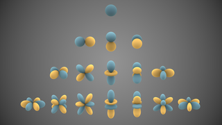
In mathematics and physical science, spherical harmonics are special functions defined on the surface of a sphere. They are often employed in solving partial differential equations in many scientific fields. The table of spherical harmonics contains a list of common spherical harmonics.

In mathematics, the Fourier inversion theorem says that for many types of functions it is possible to recover a function from its Fourier transform. Intuitively it may be viewed as the statement that if we know all frequency and phase information about a wave then we may reconstruct the original wave precisely.

In mathematics, the Mellin transform is an integral transform that may be regarded as the multiplicative version of the two-sided Laplace transform. This integral transform is closely connected to the theory of Dirichlet series, and is often used in number theory, mathematical statistics, and the theory of asymptotic expansions; it is closely related to the Laplace transform and the Fourier transform, and the theory of the gamma function and allied special functions.

In mathematics, the Riesz–Thorin theorem, often referred to as the Riesz–Thorin interpolation theorem or the Riesz–Thorin convexity theorem, is a result about interpolation of operators. It is named after Marcel Riesz and his student G. Olof Thorin.

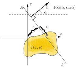
In mathematics, in the area of harmonic analysis, the fractional Fourier transform (FRFT) is a family of linear transformations generalizing the Fourier transform. It can be thought of as the Fourier transform to the n-th power, where n need not be an integer — thus, it can transform a function to any intermediate domain between time and frequency. Its applications range from filter design and signal analysis to phase retrieval and pattern recognition.

In calculus, the Leibniz integral rule for differentiation under the integral sign states that for an integral of the form

In mathematics, in particular in algebraic geometry and differential geometry, Dolbeault cohomology (named after Pierre Dolbeault) is an analog of de Rham cohomology for complex manifolds. Let M be a complex manifold. Then the Dolbeault cohomology groups depend on a pair of integers p and q and are realized as a subquotient of the space of complex differential forms of degree (p,q).

In many-body theory, the term Green's function is sometimes used interchangeably with correlation function, but refers specifically to correlators of field operators or creation and annihilation operators.

<span class="mw-page-title-main">Dirichlet kernel</span> Concept in mathematical analysis

In mathematical analysis, the Dirichlet kernel, named after the German mathematician Peter Gustav Lejeune Dirichlet, is the collection of periodic functions defined as

The Mehler kernel is a complex-valued function found to be the propagator of the quantum harmonic oscillator.

In optics, the Fraunhofer diffraction equation is used to model the diffraction of waves when the diffraction pattern is viewed at a long distance from the diffracting object, and also when it is viewed at the focal plane of an imaging lens.

In mathematics, the oscillator representation is a projective unitary representation of the symplectic group, first investigated by Irving Segal, David Shale, and André Weil. A natural extension of the representation leads to a semigroup of contraction operators, introduced as the oscillator semigroup by Roger Howe in 1988. The semigroup had previously been studied by other mathematicians and physicists, most notably Felix Berezin in the 1960s. The simplest example in one dimension is given by SU(1,1). It acts as Möbius transformations on the extended complex plane, leaving the unit circle invariant. In that case the oscillator representation is a unitary representation of a double cover of SU(1,1) and the oscillator semigroup corresponds to a representation by contraction operators of the semigroup in SL(2,C) corresponding to Möbius transformations that take the unit disk into itself.

Fractional wavelet transform (FRWT) is a generalization of the classical wavelet transform (WT). This transform is proposed in order to rectify the limitations of the WT and the fractional Fourier transform (FRFT). The FRWT inherits the advantages of multiresolution analysis of the WT and has the capability of signal representations in the fractional domain which is similar to the FRFT.

Lightfieldmicroscopy (LFM) is a scanning-free 3-dimensional (3D) microscopic imaging method based on the theory of light field. This technique allows sub-second (~10 Hz) large volumetric imaging with ~1 μm spatial resolution in the condition of weak scattering and semi-transparence, which has never been achieved by other methods. Just as in traditional light field rendering, there are two steps for LFM imaging: light field capture and processing. In most setups, a microlens array is used to capture the light field. As for processing, it can be based on two kinds of representations of light propagation: the ray optics picture and the wave optics picture. The Stanford University Computer Graphics Laboratory published their first prototype LFM in 2006 and has been working on the cutting edge since then.

References

Further reading