Rule of succession

This article is about the rule of succession in probability theory. For monarchical and presidential rules of succession, see Order of succession.

"Laplace–Bayes estimator" redirects here. For statistical estimators that maximize posterior expected utility or minimize posterior expected loss, see Bayes estimator.

In probability theory, the rule of succession is a formula introduced in the 18th century by Pierre-Simon Laplace in the course of treating the sunrise problem. ^[1] The formula is still used, particularly to estimate underlying probabilities when there are few observations or events that have not been observed to occur at all in (finite) sample data.

Statement of the rule of succession

If we repeat an experiment that we know can result in a success or failure, n times independently, and get s successes, and n − s failures, then what is the probability that the next repetition will succeed?

More abstractly: If X₁, ..., X_n+1 are conditionally independent random variables that each can assume the value 0 or 1, then, if we know nothing more about them,

${\displaystyle P(X_{n+1}=1\mid X_{1}+\cdots +X_{n}=s)={s+1 \over n+2}.}$

Interpretation

Since we have the prior knowledge that we are looking at an experiment for which both success and failure are possible, our estimate is as if we had observed one success and one failure for sure before we even started the experiments. In a sense we made n + 2 observations (known as pseudocounts) with s + 1 successes. Although this may seem the simplest and most reasonable assumption, which also happens to be true, it still requires a proof. Indeed, assuming a pseudocount of one per possibility is one way to generalise the binary result, but has unexpected consequences — see Generalization to any number of possibilities, below.

Nevertheless, if we had not known from the start that both success and failure are possible, then we would have had to assign

${\displaystyle P'(X_{n+1}=1\mid X_{1}+\cdots +X_{n}=s)={s \over n}.}$

But see Mathematical details, below, for an analysis of its validity. In particular it is not valid when ${\displaystyle s=0}$, or ${\displaystyle s=n}$.

If the number of observations increases, ${\displaystyle P}$ and ${\displaystyle P'}$ get more and more similar, which is intuitively clear: the more data we have, the less importance should be assigned to our prior information.

Historical application to the sunrise problem

Laplace used the rule of succession to calculate the probability that the Sun will rise tomorrow, given that it has risen every day for the past 5000 years. One obtains a very large factor of approximately 5000 × 365.25, which gives odds of about 1,826,200 to 1 in favour of the Sun rising tomorrow.

However, as the mathematical details below show, the basic assumption for using the rule of succession would be that we have no prior knowledge about the question whether the Sun will or will not rise tomorrow, except that it can do either. This is not the case for sunrises.

Laplace knew this well, and he wrote to conclude the sunrise example: "But this number is far greater for him who, seeing in the totality of phenomena the principle regulating the days and seasons, realizes that nothing at the present moment can arrest the course of it." ^[2] Yet Laplace was ridiculed for this calculation; his opponents^{[ who? ]} gave no heed to that sentence, or failed to understand its importance. ^[2]

In the 1940s, Rudolf Carnap investigated a probability-based theory of inductive reasoning, and developed measures of degree of confirmation, which he considered as alternatives to Laplace's rule of succession. ^{[3] [4]} See also New riddle of induction#Carnap.

Intuition

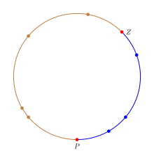
The point Z is the zero point, P is the point such that the fraction of the circle from Z to P (in blue) is equal to p. The value of p is precisely the number of blue arcs divided by the total number of arcs. If we let the first clockwise point of an arc define it, then every point on the circle defines one arc with Z defining a blue arc and P defining a non-blue arc. The estimate for p is then one (Z) more than blue points divided by two (Z and P) more than total number of trials which is the rule of succession.

The rule of succession can be interpreted in an intuitive manner by considering points randomly distributed on a circle rather than counting the number "success"/"failures" in an experiment. ^[5] To mimic the behavior of the proportion p on the circle, we will color the circle in two colors and the fraction of the circle colored in the "success" color will be equal to p. To express the uncertainty about the value of p, we need to select a fraction of the circle.

A fraction is chosen by selecting two uniformly random points on the circle. The first point Z corresponds to the zero in the [0, 1] interval and the second point P corresponds to p within [0, 1]. In terms of the circle the fraction of the circle from Z to P moving clockwise will be equal to p. The n trials can be interpreted as n points uniformly distributed on the circle; any point in the "success" fraction is a success and a failure otherwise. This provides an exact mapping from success/failure experiments with probability of success p to uniformly random points on the circle. In the figure the success fraction is colored blue to differentiate it from the rest of the circle and the points P and Z are highlighted in red.

Given this circle, the estimate of p is the fraction colored blue. Let us divide the circle into n+2 arcs corresponding to the n+2 points such that the portion from a point on the circle to the next point (moving clockwise) is one arc associated with the first point. Thus, Z defines the first blue arc while P defines the first non-blue/failure arc. Since the next point is a uniformly random point, if it falls in any of the blue arcs then the trial succeeds while if it falls in any of the other arcs, then it fails. So the probability of success p is ${\displaystyle {\frac {b}{t}}}$ where b is the number of blue arcs and t is the total number of arcs. Note that there is one more blue arc (that of Z) than success point and two more arcs (those of P and Z) than n points. Substituting the values with number of successes gives the rule of succession.

Note: The actual probability needs to use the length of blue arcs divided by the length of all arcs. However, when k points are uniformly randomly distributed on a circle, the distance from a point to the next point is 1/k. So on average each arc is of the same length and ratio of lengths becomes ratio of counts.

Mathematical details

The proportion p is assigned a uniform distribution to describe the uncertainty about its true value. (This proportion is not random, but uncertain. We assign a probability distribution to p to express our uncertainty, not to attribute randomness to p. But this amounts, mathematically, to the same thing as treating p as if it were random).

Let X_i be 1 if we observe a "success" on the ith trial, otherwise 0, with probability p of success on each trial. Thus each X is 0 or 1; each X has a Bernoulli distribution. Suppose these Xs are conditionally independent given p.

We can use Bayes' theorem to find the conditional probability distribution of p given the data X_i, i = 1, ..., n. For the "prior" (i.e., marginal) probability measure of p we assigned a uniform distribution over the open interval (0,1)

${\displaystyle f(p)={\begin{cases}0&{\text{for }}p\leq 0\\1&{\text{for }}0<p<1\\0&{\text{for }}p\geq 1\end{cases}}}$

For the likelihood of a given p under our observations, we use the likelihood function

${\displaystyle L(p)=P(X_{1}=x_{1},\ldots ,X_{n}=x_{n}\mid p)=\prod _{i=1}^{n}p^{x_{i}}(1-p)^{1-x_{i}}=p^{s}(1-p)^{n-s}}$

where s = x₁ + ... + x_n is the number of "successes" and n is the number of trials (we are using capital X to denote a random variable and lower-case x as the data actually observed). Putting it all together, we can calculate the posterior:

${\displaystyle f(p\mid X_{1}=x_{1},\ldots ,X_{n}=x_{n})={L(p)f(p) \over \int _{0}^{1}L(r)f(r)\,dr}={p^{s}(1-p)^{n-s} \over \int _{0}^{1}r^{s}(1-r)^{n-s}\,dr}}$

To get the normalizing constant, we find

${\displaystyle \int _{0}^{1}r^{s}(1-r)^{n-s}\,dr={s!(n-s)! \over (n+1)!}}$

(see beta function for more on integrals of this form).

The posterior probability density function is therefore

${\displaystyle f(p\mid X_{1}=x_{1},\ldots ,X_{n}=x_{n})={(n+1)! \over s!(n-s)!}p^{s}(1-p)^{n-s}.}$

This is a beta distribution with expected value

${\displaystyle \operatorname {E} (p\mid X_{i}=x_{i}{\text{ for }}i=1,\dots ,n)=\int _{0}^{1}pf(p\mid X_{1}=x_{1},\ldots ,X_{n}=x_{n})\,dp={s+1 \over n+2}.}$

Since p tells us the probability of success in any experiment, and each experiment is conditionally independent, the conditional probability for success in the next experiment is just p. As p is being treated as if it is a random variable, the law of total probability tells us that the expected probability of success in the next experiment is just the expected value of p. Since p is conditional on the observed data X_i for i = 1, ..., n, we have

${\displaystyle P(X_{n+1}=1\mid X_{i}=x_{i}{\text{ for }}i=1,\dots ,n)=\operatorname {E} (p\mid X_{i}=x_{i}{\text{ for }}i=1,\dots ,n)={s+1 \over n+2}.}$

The same calculation can be performed with the (improper) prior that expresses total ignorance of p, including ignorance with regard to the question whether the experiment can succeed, or can fail. This improper prior is 1/(p(1 − p)) for 0 ≤ p ≤ 1 and 0 otherwise. ^[6] If the calculation above is repeated with this prior, we get

${\displaystyle P'(X_{n+1}=1\mid X_{i}=x_{i}{\text{ for }}i=1,\dots ,n)={s \over n}.}$

Thus, with the prior specifying total ignorance, the probability of success is governed by the observed frequency of success. However, the posterior distribution that led to this result is the Beta(s,n − s) distribution, which is not proper when s = n or s = 0 (i.e. the normalisation constant is infinite when s = 0 or s = n). This means that we cannot use this form of the posterior distribution to calculate the probability of the next observation succeeding when s = 0 or s = n. This puts the information contained in the rule of succession in greater light: it can be thought of as expressing the prior assumption that if sampling was continued indefinitely, we would eventually observe at least one success, and at least one failure in the sample. The prior expressing total ignorance does not assume this knowledge.

To evaluate the "complete ignorance" case when s = 0 or s = n can be dealt with, we first go back to the hypergeometric distribution, denoted by ${\displaystyle \mathrm {Hyp} (s|N,n,S)}$. This is the approach taken in Jaynes (2003). The binomial Failed to parse (SVG (MathML can be enabled via browser plugin): Invalid response ("Math extension cannot connect to Restbase.") from server "http://localhost:6011/en.wikipedia.org/v1/":): {\mathrm {Bin}}(r|n,p) can be derived as a limiting form, where ${\displaystyle N,S\rightarrow \infty }$ in such a way that their ratio ${\displaystyle p={S \over N}}$ remains fixed. One can think of ${\displaystyle S}$ as the number of successes in the total population, of size ${\displaystyle N}$.

The equivalent prior to ${\displaystyle {1 \over p(1-p)}}$ is ${\displaystyle {1 \over S(N-S)}}$, with a domain of ${\displaystyle 1\leq S\leq N-1}$. Working conditional to ${\displaystyle N}$ means that estimating ${\displaystyle p}$ is equivalent to estimating ${\displaystyle S}$, and then dividing this estimate by ${\displaystyle N}$. The posterior for ${\displaystyle S}$ can be given as:

${\displaystyle P(S|N,n,s)\propto {1 \over S(N-S)}{S \choose s}{N-S \choose n-s}\propto {S!(N-S)! \over S(N-S)(S-s)!(N-S-[n-s])!}}$

And it can be seen that, if s = n or s = 0, then one of the factorials in the numerator cancels exactly with one in the denominator. Taking the s = 0 case, we have:

${\displaystyle P(S|N,n,s=0)\propto {(N-S-1)! \over S(N-S-n)!}={\prod _{j=1}^{n-1}(N-S-j) \over S}}$

Adding in the normalising constant, which is always finite (because there are no singularities in the range of the posterior, and there are a finite number of terms) gives:

${\displaystyle P(S|N,n,s=0)={\prod _{j=1}^{n-1}(N-S-j) \over S\sum _{R=1}^{N-n}{\prod _{j=1}^{n-1}(N-R-j) \over R}}}$

So the posterior expectation for ${\displaystyle p={S \over N}}$ is:

${\displaystyle E\left({S \over N}|n,s=0,N\right)={1 \over N}\sum _{S=1}^{N-n}SP(S|N,n=1,s=0)={1 \over N}{\sum _{S=1}^{N-n}\prod _{j=1}^{n-1}(N-S-j) \over \sum _{R=1}^{N-n}{\prod _{j=1}^{n-1}(N-R-j) \over R}}}$

An approximate analytical expression for large N is given by first making the approximation to the product term:

${\displaystyle \prod _{j=1}^{n-1}(N-R-j)\approx (N-R)^{n-1}}$

and then replacing the summation in the numerator with an integral

${\displaystyle \sum _{S=1}^{N-n}\prod _{j=1}^{n-1}(N-S-j)\approx \int _{1}^{N-n}(N-S)^{n-1}\,dS={(N-1)^{n}-n^{n} \over n}\approx {N^{n} \over n}}$

The same procedure is followed for the denominator, but the process is a bit more tricky, as the integral is harder to evaluate

${\displaystyle {\begin{aligned}\sum _{R=1}^{N-n}{\prod _{j=1}^{n-1}(N-R-j) \over R}&\approx \int _{1}^{N-n}{(N-R)^{n-1} \over R}\,dR\\&=N\int _{1}^{N-n}{(N-R)^{n-2} \over R}\,dR-\int _{1}^{N-n}(N-R)^{n-2}\,dR\\&=N^{n-1}\left[\int _{1}^{N-n}{dR \over R}-{1 \over n-1}+O\left({1 \over N}\right)\right]\approx N^{n-1}\ln(N)\end{aligned}}}$

where ln is the natural logarithm plugging in these approximations into the expectation gives

${\displaystyle E\left({S \over N}|n,s=0,N\right)\approx {1 \over N}{{N^{n} \over n} \over N^{n-1}\ln(N)}={1 \over n[\ln(N)]}={\log _{10}(e) \over n[\log _{10}(N)]}={0.434294 \over n[\log _{10}(N)]}}$

where the base 10 logarithm has been used in the final answer for ease of calculation. For instance if the population is of size 10^k then probability of success on the next sample is given by:

${\displaystyle E\left({S \over N}\mid n,s=0,N=10^{k}\right)\approx {0.434294 \over nk}}$

So for example, if the population be on the order of tens of billions, so that k = 10, and we observe n = 10 results without success, then the expected proportion in the population is approximately 0.43%. If the population is smaller, so that n = 10, k = 5 (tens of thousands), the expected proportion rises to approximately 0.86%, and so on. Similarly, if the number of observations is smaller, so that n = 5, k = 10, the proportion rise to approximately 0.86% again.

This probability has no positive lower bound, and can be made arbitrarily small for larger and larger choices of N, or k. This means that the probability depends on the size of the population from which one is sampling. In passing to the limit of infinite N (for the simpler analytic properties) we are "throwing away" a piece of very important information. Note that this ignorance relationship only holds as long as only no successes are observed. It is correspondingly revised back to the observed frequency rule ${\displaystyle p={s \over n}}$ as soon as one success is observed. The corresponding results are found for the s=n case by switching labels, and then subtracting the probability from 1.

Generalization to any number of possibilities

This section gives a heuristic derivation similar to that in Probability Theory: The Logic of Science. ^[7]

The rule of succession has many different intuitive interpretations, and depending on which intuition one uses, the generalisation may be different. Thus, the way to proceed from here is very carefully, and to re-derive the results from first principles, rather than to introduce an intuitively sensible generalisation. The full derivation can be found in Jaynes' book, but it does admit an easier to understand alternative derivation, once the solution is known. Another point to emphasise is that the prior state of knowledge described by the rule of succession is given as an enumeration of the possibilities, with the additional information that it is possible to observe each category. This can be equivalently stated as observing each category once prior to gathering the data. To denote that this is the knowledge used, an I_m is put as part of the conditions in the probability assignments.

The rule of succession comes from setting a binomial likelihood, and a uniform prior distribution. Thus a straightforward generalisation is just the multivariate extensions of these two distributions: 1) Setting a uniform prior over the initial m categories, and 2) using the multinomial distribution as the likelihood function (which is the multivariate generalisation of the binomial distribution). It can be shown that the uniform distribution is a special case of the Dirichlet distribution with all of its parameters equal to 1 (just as the uniform is Beta(1,1) in the binary case). The Dirichlet distribution is the conjugate prior for the multinomial distribution, which means that the posterior distribution is also a Dirichlet distribution with different parameters. Let p_i denote the probability that category i will be observed, and let n_i denote the number of times category i (i = 1, ..., m) actually was observed. Then the joint posterior distribution of the probabilities p₁, ..., p_m is given by:

${\displaystyle f(p_{1},\ldots ,p_{m}\mid n_{1},\ldots ,n_{m},I)={\begin{cases}{\displaystyle {\frac {\Gamma \left(\sum _{i=1}^{m}(n_{i}+1)\right)}{\prod _{i=1}^{m}\Gamma (n_{i}+1)}}p_{1}^{n_{1}}\cdots p_{m}^{n_{m}}},\quad &\sum _{i=1}^{m}p_{i}=1\\\\0&{\text{otherwise.}}\end{cases}}}$

To get the generalised rule of succession, note that the probability of observing category i on the next observation, conditional on the p_i is just p_i, we simply require its expectation. Letting A_i denote the event that the next observation is in category i (i = 1, ..., m), and let n = n₁ + ... + n_m be the total number of observations made. The result, using the properties of the Dirichlet distribution is:

${\displaystyle P(A_{i}|n_{1},\ldots ,n_{m},I_{m})={n_{i}+1 \over n+m}.}$

This solution reduces to the probability that would be assigned using the principle of indifference before any observations made (i.e. n = 0), consistent with the original rule of succession. It also contains the rule of succession as a special case, when m = 2, as a generalisation should.

Because the propositions or events A_i are mutually exclusive, it is possible to collapse the m categories into 2. Simply add up the A_i probabilities that correspond to "success" to get the probability of success. Supposing that this aggregates c categories as "success" and m-c categories as "failure". Let s denote the sum of the relevant n_i values that have been termed "success". The probability of "success" at the next trial is then:

${\displaystyle P({\text{success}}|n_{1},\ldots ,n_{m},I_{m})={s+c \over n+m},}$

which is different from the original rule of succession. But note that the original rule of succession is based on I₂, whereas the generalisation is based on I_m. This means that the information contained in I_m is different from that contained in I₂. This indicates that mere knowledge of more than two outcomes we know are possible is relevant information when collapsing these categories down to just two. This illustrates the subtlety in describing the prior information, and why it is important to specify which prior information one is using.

Further analysis

A good model is essential (i.e., a good compromise between accuracy and practicality). To paraphrase Laplace on the sunrise problem: Although we have a huge number of samples of the sun rising, there are far better models of the sun than assuming it has a certain probability of rising each day, e.g., simply having a half-life.

Given a good model, it is best to make as many observations as practicable, depending on the expected reliability of prior knowledge, cost of observations, time and resources available, and accuracy required.

One of the most difficult aspects of the rule of succession is not the mathematical formulas, but answering the question: When does the rule of succession apply? In the generalisation section, it was noted very explicitly by adding the prior information I_m into the calculations. Thus, when all that is known about a phenomenon is that there are m known possible outcomes prior to observing any data, only then does the rule of succession apply. If the rule of succession is applied in problems where this does not accurately describe the prior state of knowledge, then it may give counter-intuitive results. This is not because the rule of succession is defective, but that it is effectively answering a different question, based on different prior information.

In principle (see Cromwell's rule), no possibility should have its probability (or its pseudocount) set to zero, since nothing in the physical world should be assumed strictly impossible (though it may be)—even if contrary to all observations and current theories. Indeed, Bayes rule takes absolutely no account of an observation previously believed to have zero probability—it is still declared impossible. However, only considering a fixed set of the possibilities is an acceptable route, one just needs to remember that the results are conditional on (or restricted to) the set being considered, and not some "universal" set. In fact Larry Bretthorst shows that including the possibility of "something else" into the hypothesis space makes no difference to the relative probabilities of the other hypothesis—it simply renormalises them to add up to a value less than 1. ^[8] Until "something else" is specified, the likelihood function conditional on this "something else" is indeterminate, for how is one to determine ${\displaystyle Pr({\text{data}}|{\text{something else}},I)}$? Thus no updating of the prior probability for "something else" can occur until it is more accurately defined.

However, it is sometimes debatable whether prior knowledge should affect the relative probabilities, or also the total weight of the prior knowledge compared to actual observations. This does not have a clear cut answer, for it depends on what prior knowledge one is considering. In fact, an alternative prior state of knowledge could be of the form "I have specified m potential categories, but I am sure that only one of them is possible prior to observing the data. However, I do not know which particular category this is." A mathematical way to describe this prior is the Dirichlet distribution with all parameters equal to m⁻¹, which then gives a pseudocount of 1 to the denominator instead of m, and adds a pseudocount of m⁻¹ to each category. This gives a slightly different probability in the binary case of ${\displaystyle {\frac {s+0.5}{n+1}}}$.

Prior probabilities are only worth spending significant effort estimating when likely to have significant effect. They may be important when there are few observations — especially when so few that there have been few, if any, observations of some possibilities – such as a rare animal, in a given region. Also important when there are many observations, where it is believed that the expectation should be heavily weighted towards the prior estimates, in spite of many observations to the contrary, such as for a roulette wheel in a well-respected casino. In the latter case, at least some of the pseudocounts may need to be very large. They are not always small, and thereby soon outweighed by actual observations, as is often assumed. However, although a last resort, for everyday purposes, prior knowledge is usually vital. So most decisions must be subjective to some extent (dependent upon the analyst and analysis used).

See also

• Additive smoothing
• Krichevsky–Trofimov estimator
• Principle of indifference

References

1. Laplace, Pierre-Simon (1814). Essai philosophique sur les probabilités. Paris: Courcier.
2. Part II Section 18.6 of Jaynes, E. T. & Bretthorst, G. L. (2003). Probability Theory: The Logic of Science. Cambridge University Press. ISBN   978-0-521-59271-0
3. Rudolf Carnap (1945). "On Inductive Logic" (PDF). Philosophy of Science. 12 (2): 72–97. doi:10.1086/286851. S2CID   14481246.; here: p.86, 97
4. Rudolf Carnap (1947). "On the Application of Inductive Logic" (PDF). Philosophy and Phenomenological Research. 8 (1): 133–148. doi:10.2307/2102920. JSTOR   2102920.; here: p.145
5. Neyman, Eric. "An elegant proof of Laplace's rule of succession". Unexpected Values. Eric Neyman. Retrieved 13 April 2023.
6. http://www.stats.org.uk/priors/noninformative/Smith.pdf ^{[ bare URL PDF ]}
7. Jaynes, E.T. (2003), Probability Theory: The Logic of Science, Cambridge, UK, Cambridge University Press.
8. Bretthost, G. Larry (1988). Bayesian Spectrum Analysis and parameter estimation (PDF) (PhD thesis). p. 55.