Principle of indifference

Last updated

The principle of indifference (also called principle of insufficient reason) is a rule for assigning epistemic probabilities. The principle of indifference states that in the absence of any relevant evidence, agents should distribute their credence (or "degrees of belief") equally among all the possible outcomes under consideration. [1]

Contents

In Bayesian probability, this is the simplest non-informative prior. The principle of indifference is meaningless under the frequency interpretation of probability,[ citation needed ] in which probabilities are relative frequencies rather than degrees of belief in uncertain propositions, conditional upon state information.

Examples

The textbook examples for the application of the principle of indifference are coins, dice, and cards.

In a macroscopic system, at least, it must be assumed that the physical laws that govern the system are not known well enough to predict the outcome. As observed some centuries ago by John Arbuthnot (in the preface of Of the Laws of Chance, 1692),

It is impossible for a Die, with such determin'd force and direction, not to fall on such determin'd side, only I don't know the force and direction which makes it fall on such determin'd side, and therefore I call it Chance, which is nothing but the want of art....

Given enough time and resources, there is no fundamental reason to suppose that suitably precise measurements could not be made, which would enable the prediction of the outcome of coins, dice, and cards with high accuracy: Persi Diaconis's work with coin-flipping machines is a practical example of this. [2]

Coins

A symmetric coin has two sides, arbitrarily labeled heads (many coins have the head of a person portrayed on one side) and tails. Assuming that the coin must land on one side or the other, the outcomes of a coin toss are mutually exclusive, exhaustive, and interchangeable. According to the principle of indifference, we assign each of the possible outcomes a probability of 1/2.

It is implicit in this analysis that the forces acting on the coin are not known with any precision. If the momentum imparted to the coin as it is launched were known with sufficient accuracy, the flight of the coin could be predicted according to the laws of mechanics. Thus the uncertainty in the outcome of a coin toss is derived (for the most part) from the uncertainty with respect to initial conditions. This point is discussed at greater length in the article on coin flipping.

Dice

A symmetric die has n faces, arbitrarily labeled from 1 to n. An ordinary cubical die has n = 6 faces, although a symmetric die with different numbers of faces can be constructed; see Dice. We assume that the die will land with one face or another upward, and there are no other possible outcomes. Applying the principle of indifference, we assign each of the possible outcomes a probability of 1/n. As with coins, it is assumed that the initial conditions of throwing the dice are not known with enough precision to predict the outcome according to the laws of mechanics. Dice are typically thrown so as to bounce on a table or other surface(s). This interaction makes prediction of the outcome much more difficult.

The assumption of symmetry is crucial here. Suppose that we are asked to bet for or against the outcome "6". We might reason that there are two relevant outcomes here "6" or "not 6", and that these are mutually exclusive and exhaustive. A common fallacy is assigning the probability 1/2 to each of the two outcomes, when "not 6" is five times more likely than "6."

Cards

A standard deck contains 52 cards, each given a unique label in an arbitrary fashion, i.e. arbitrarily ordered. We draw a card from the deck; applying the principle of indifference, we assign each of the possible outcomes a probability of 1/52.

This example, more than the others, shows the difficulty of actually applying the principle of indifference in real situations. What we really mean by the phrase "arbitrarily ordered" is simply that we don't have any information that would lead us to favor a particular card. In actual practice, this is rarely the case: a new deck of cards is certainly not in arbitrary order, and neither is a deck immediately after a hand of cards. In practice, we therefore shuffle the cards; this does not destroy the information we have, but instead (hopefully) renders our information practically unusable, although it is still usable in principle. In fact, some expert blackjack players can track aces through the deck; for them, the condition for applying the principle of indifference is not satisfied.

Application to continuous variables

Applying the principle of indifference incorrectly can easily lead to nonsensical results, especially in the case of multivariate, continuous variables. A typical case of misuse is the following example:

In this example, mutually contradictory estimates of the length, surface area, and volume of the cube arise because we have assumed three mutually contradictory distributions for these parameters: a uniform distribution for any one of the variables implies a non-uniform distribution for the other two. In general, the principle of indifference does not indicate which variable (e.g. in this case, length, surface area, or volume) is to have a uniform epistemic probability distribution.

Another classic example of this kind of misuse is the Bertrand paradox. Edwin T. Jaynes introduced the principle of transformation groups, which can yield an epistemic probability distribution for this problem. This generalises the principle of indifference, by saying that one is indifferent between equivalent problems rather than indifferent between propositions. This still reduces to the ordinary principle of indifference when one considers a permutation of the labels as generating equivalent problems (i.e. using the permutation transformation group). To apply this to the above box example, we have three random variables related by geometric equations. If we have no reason to favour one trio of values over another, then our prior probabilities must be related by the rule for changing variables in continuous distributions. Let L be the length, and V be the volume. Then we must have

,

where are the probability density functions (pdf) of the stated variables. This equation has a general solution: , where K is a normalization constant, determined by the range of L, in this case equal to:

To put this "to the test", we ask for the probability that the length is less than 4. This has probability of:

.

For the volume, this should be equal to the probability that the volume is less than 43 = 64. The pdf of the volume is

.

And then probability of volume less than 64 is

.

Thus we have achieved invariance with respect to volume and length. One can also show the same invariance with respect to surface area being less than 6(42) = 96. However, note that this probability assignment is not necessarily a "correct" one. For the exact distribution of lengths, volume, or surface area will depend on how the "experiment" is conducted.

The fundamental hypothesis of statistical physics, that any two microstates of a system with the same total energy are equally probable at equilibrium, is in a sense an example of the principle of indifference. However, when the microstates are described by continuous variables (such as positions and momenta), an additional physical basis is needed in order to explain under which parameterization the probability density will be uniform. Liouville's theorem justifies the use of canonically conjugate variables, such as positions and their conjugate momenta.

The wine/water paradox shows a dilemma with linked variables, and which one to choose.

History

This principle stems from Epicurus' principle of "multiple explanations" (pleonachos tropos), [3] according to which "if more than one theory is consistent with the data, keep them all”. The epicurean Lucretius developed this point with an analogy of the multiple causes of death of a corpse. [4] The original writers on probability, primarily Jacob Bernoulli and Pierre Simon Laplace, considered the principle of indifference to be intuitively obvious and did not even bother to give it a name. Laplace wrote:

The theory of chance consists in reducing all the events of the same kind to a certain number of cases equally possible, that is to say, to such as we may be equally undecided about in regard to their existence, and in determining the number of cases favorable to the event whose probability is sought. The ratio of this number to that of all the cases possible is the measure of this probability, which is thus simply a fraction whose numerator is the number of favorable cases and whose denominator is the number of all the cases possible.

These earlier writers, Laplace in particular, naively generalized the principle of indifference to the case of continuous parameters, giving the so-called "uniform prior probability distribution", a function that is constant over all real numbers. He used this function to express a complete lack of knowledge as to the value of a parameter. According to Stigler (page 135), Laplace's assumption of uniform prior probabilities was not a meta-physical assumption. [5] It was an implicit assumption made for the ease of analysis.

The principle of insufficient reason was its first name, given to it by Johannes von Kries, [6] possibly as a play on Leibniz's principle of sufficient reason. These later writers (George Boole, John Venn, and others) objected to the use of the uniform prior for two reasons. The first reason is that the constant function is not normalizable, and thus is not a proper probability distribution. The second reason is its inapplicability to continuous variables, as described above.

The "principle of insufficient reason" was renamed the "principle of indifference" by John MaynardKeynes  ( 1921 ), [7] who was careful to note that it applies only when there is no knowledge indicating unequal probabilities.

Attempts to put the notion on firmer philosophical ground have generally begun with the concept of equipossibility and progressed from it to equiprobability.

The principle of indifference can be given a deeper logical justification by noting that equivalent states of knowledge should be assigned equivalent epistemic probabilities. This argument was propounded by Edwin Thompson Jaynes: it leads to two generalizations, namely the principle of transformation groups as in the Jeffreys prior, and the principle of maximum entropy. [8]

More generally, one speaks of uninformative priors.

See also

Related Research Articles

Information theory is the mathematical study of the quantification, storage, and communication of information. The field was originally established by the works of Harry Nyquist and Ralph Hartley, in the 1920s, and Claude Shannon in the 1940s. The field, in applied mathematics, is at the intersection of probability theory, statistics, computer science, statistical mechanics, information engineering, and electrical engineering.

<span class="mw-page-title-main">Entropy (information theory)</span> Expected amount of information needed to specify the output of a stochastic data source

In information theory, the entropy of a random variable is the average level of "information", "surprise", or "uncertainty" inherent to the variable's possible outcomes. Given a discrete random variable , which takes values in the alphabet and is distributed according to , the entropy is

<span class="mw-page-title-main">Probability theory</span> Branch of mathematics concerning probability

Probability theory or probability calculus is the branch of mathematics concerned with probability. Although there are several different probability interpretations, probability theory treats the concept in a rigorous mathematical manner by expressing it through a set of axioms. Typically these axioms formalise probability in terms of a probability space, which assigns a measure taking values between 0 and 1, termed the probability measure, to a set of outcomes called the sample space. Any specified subset of the sample space is called an event.

<span class="mw-page-title-main">Probability distribution</span> Mathematical function for the probability a given outcome occurs in an experiment

In probability theory and statistics, a probability distribution is the mathematical function that gives the probabilities of occurrence of different possible outcomes for an experiment. It is a mathematical description of a random phenomenon in terms of its sample space and the probabilities of events.

<span class="mw-page-title-main">Random variable</span> Variable representing a random phenomenon

A random variable is a mathematical formalization of a quantity or object which depends on random events. The term 'random variable' can be misleading as its mathematical definition is not actually random nor a variable, but rather it is a function from possible outcomes in a sample space to a measurable space, often to the real numbers.

<span class="mw-page-title-main">Probability space</span> Mathematical concept

In probability theory, a probability space or a probability triple is a mathematical construct that provides a formal model of a random process or "experiment". For example, one can define a probability space which models the throwing of a die.

<span class="mw-page-title-main">Bernoulli process</span> Random process of binary (boolean) random variables

In probability and statistics, a Bernoulli process is a finite or infinite sequence of binary random variables, so it is a discrete-time stochastic process that takes only two values, canonically 0 and 1. The component Bernoulli variablesXi are identically distributed and independent. Prosaically, a Bernoulli process is a repeated coin flipping, possibly with an unfair coin. Every variable Xi in the sequence is associated with a Bernoulli trial or experiment. They all have the same Bernoulli distribution. Much of what can be said about the Bernoulli process can also be generalized to more than two outcomes ; this generalization is known as the Bernoulli scheme.

<span class="mw-page-title-main">Probability mass function</span> Discrete-variable probability distribution

In probability and statistics, a probability mass function is a function that gives the probability that a discrete random variable is exactly equal to some value. Sometimes it is also known as the discrete probability density function. The probability mass function is often the primary means of defining a discrete probability distribution, and such functions exist for either scalar or multivariate random variables whose domain is discrete.

<span class="mw-page-title-main">Law of large numbers</span> Averages of repeated trials converge to the expected value

In probability theory, the law of large numbers (LLN) is a mathematical theorem that states that the average of the results obtained from a large number of independent and identical random samples converges to the true value, if it exists. More formally, the LLN states that given a sample of independent and identically distributed values, the sample mean converges to the true mean.

The principle of maximum entropy states that the probability distribution which best represents the current state of knowledge about a system is the one with largest entropy, in the context of precisely stated prior data.

<span class="mw-page-title-main">Logistic regression</span> Statistical model for a binary dependent variable

In statistics, the logistic model is a statistical model that models the log-odds of an event as a linear combination of one or more independent variables. In regression analysis, logistic regression is estimating the parameters of a logistic model. Formally, in binary logistic regression there is a single binary dependent variable, coded by an indicator variable, where the two values are labeled "0" and "1", while the independent variables can each be a binary variable or a continuous variable. The corresponding probability of the value labeled "1" can vary between 0 and 1, hence the labeling; the function that converts log-odds to probability is the logistic function, hence the name. The unit of measurement for the log-odds scale is called a logit, from logistic unit, hence the alternative names. See § Background and § Definition for formal mathematics, and § Example for a worked example.

A prior probability distribution of an uncertain quantity, often simply called the prior, is its assumed probability distribution before some evidence is taken into account. For example, the prior could be the probability distribution representing the relative proportions of voters who will vote for a particular politician in a future election. The unknown quantity may be a parameter of the model or a latent variable rather than an observable variable.

In information theory, the information content, self-information, surprisal, or Shannon information is a basic quantity derived from the probability of a particular event occurring from a random variable. It can be thought of as an alternative way of expressing probability, much like odds or log-odds, but which has particular mathematical advantages in the setting of information theory.

<span class="mw-page-title-main">Continuous uniform distribution</span> Uniform distribution on an interval

In probability theory and statistics, the continuous uniform distributions or rectangular distributions are a family of symmetric probability distributions. Such a distribution describes an experiment where there is an arbitrary outcome that lies between certain bounds. The bounds are defined by the parameters, and which are the minimum and maximum values. The interval can either be closed or open. Therefore, the distribution is often abbreviated where stands for uniform distribution. The difference between the bounds defines the interval length; all intervals of the same length on the distribution's support are equally probable. It is the maximum entropy probability distribution for a random variable under no constraint other than that it is contained in the distribution's support.

In statistics and information theory, a maximum entropy probability distribution has entropy that is at least as great as that of all other members of a specified class of probability distributions. According to the principle of maximum entropy, if nothing is known about a distribution except that it belongs to a certain class, then the distribution with the largest entropy should be chosen as the least-informative default. The motivation is twofold: first, maximizing entropy minimizes the amount of prior information built into the distribution; second, many physical systems tend to move towards maximal entropy configurations over time.

In Bayesian probability, the Jeffreys prior, named after Sir Harold Jeffreys, is a non-informative prior distribution for a parameter space; its density function is proportional to the square root of the determinant of the Fisher information matrix:

In statistics, multinomial logistic regression is a classification method that generalizes logistic regression to multiclass problems, i.e. with more than two possible discrete outcomes. That is, it is a model that is used to predict the probabilities of the different possible outcomes of a categorically distributed dependent variable, given a set of independent variables.

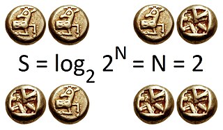
Equiprobability is a property for a collection of events that each have the same probability of occurring. In statistics and probability theory it is applied in the discrete uniform distribution and the equidistribution theorem for rational numbers. If there are events under consideration, the probability of each occurring is

In probability theory and statistics, a collection of random variables is independent and identically distributed if each random variable has the same probability distribution as the others and all are mutually independent. This property is usually abbreviated as i.i.d., iid, or IID. IID was first defined in statistics and finds application in different fields such as data mining and signal processing.

The principle of transformation groups is a methodology for assigning prior probabilities in statistical inference issues, initially proposed by E. T. Jaynes. It is regarded as an extension of the principle of indifference.

References

  1. Eva, Benjamin (30 April 2019). "Principles of Indifference". philsci-archive.pitt.edu (Preprint). Retrieved 30 September 2019.
  2. Diaconis, Persi; Keller, Joseph B. (1989). "Fair Dice". The American Mathematical Monthly. 96 (4): 337–339. doi:10.2307/2324089. JSTOR   2324089.(Discussion of dice that are fair "by symmetry" and "by continuity".)
  3. Verde, Francesco (2020-07-06). "Epicurean Meteorology, Lucretius, and the Aetna". Lucretius Poet and Philosopher. De Gruyter. pp. 83–102. doi:10.1515/9783110673487-006. ISBN   978-3-11-067348-7. S2CID   243676846.
  4. Rathmanner, Samuel; Hutter, Marcus (2011-06-03). "A Philosophical Treatise of Universal Induction". Entropy. 13 (6): 1076–1136. arXiv: 1105.5721 . Bibcode:2011Entrp..13.1076R. doi: 10.3390/e13061076 . ISSN   1099-4300.
  5. Stigler, Stephen M. (1986). The History of Statistics: The Measurement of Uncertainty Before 1900 . Cambridge, Mass: Belknap Press of Harvard University Press. ISBN   0-674-40340-1.
  6. Howson, Colin; Urbach, Peter (1989). "Subjective Probability". Scientific Reasoning : The Bayesian Approach. La Salle: Open Court. pp. 39–76. ISBN   0-8126-9084-2.
  7. Keynes, John Maynard (1921). "Chapter IV. The Principle of Indifference". A Treatise on Probability. Vol. 4. Macmillan and Co. pp. 41–64. ISBN   9780404145637.
  8. Jaynes, Edwin Thompson (2003). "Ignorance Priors and Transformation Groups". Probability Theory: The Logic of Science. Cambridge University Press. pp. 327–347. ISBN   0-521-59271-2.