Principle of transformation groups

Last updated May 14, 2024

The principle of transformation groups is a methodology for assigning prior probabilities in statistical inference issues, initially proposed by E. T. Jaynes.^[1] It is regarded as an extension of the principle of indifference.

Prior probabilities determined by this principle are objective in that they rely solely on the inherent characteristics of the problem, ensuring that any two individuals applying the principle to the same issue would assign identical prior probabilities. Thus, this principle is integral to the objective Bayesian interpretation of probability.

Motivation and Method Description

The rule is motivated by the following normative principle or desideratum:

In scenarios where the prior information is identical, individuals should assign the same prior probabilities.

The implementation of this rule involves identifying symmetries within a problem that allow it to be converted into an equivalent one, utilizing these symmetries to calculate the prior probabilities. These symmetries are defined by transformation groups.

For problems with discrete variables (such as dice, cards, or categorical data), the symmetries are characterized by permutation groups, and in these instances, the principle simplifies to the principle of indifference. In cases involving continuous variables, the symmetries may be represented by other types of transformation groups. Determining the prior probabilities in such cases often requires solving a differential equation, which may not yield a unique solution. However, many continuous variable problems do have prior probabilities uniquely defined by the principle of transformation groups, which Jaynes referred to as "well-posed" problems.

Examples

Discrete case: coin flipping

Consider a coin with head (H) and tail (T). Denote this information by I. For a given coin flip, denote the probability of an outcome of heads as $P(H|I)$ . Denote the probability of an outcome of tails by $P(T|I)$ .

In applying the desideratum, consider the information contained in the event of the coin flip as framed. It describes no distinction between heads and tails. Given no other information, the elements "head" and "tail" are interchangeable. Application of the desideratum then demands that:

P(H|I)=P(T|I)

The probabilities must add to 1, thus:

P(H|I)+P(T|I)=1\rightarrow 2P(H|I)=1\rightarrow P(H|I)=0.5

.

This argument extends to N categories, to give the "flat" prior probability 1/N.

This provides a consistency-based argument for the principle of indifference: If someone is truly ignorant about a discrete or countable set of outcomes apart from their potential existence but does not assign them equal prior probabilities, then they are assigning different probabilities when given the same information.

This can be alternatively phrased as: a person who does not use the principle of indifference to assign prior probabilities to discrete variables, is either not ignorant about them, or reasoning inconsistently.

Continuous Case: Location Parameter

This is the easiest example for continuous variables. It is given by stating one is "ignorant" of the location parameter in a given problem. The statement that a parameter is a "location parameter" is that the sampling distribution, or likelihood of an observation X depends on a parameter $\mu$ only through the difference.

p(X|\mu ,I)=f(X-\mu )

for some normalized probability distribution f(.).

Note that the given information that f(.) is a normalized distribution is a significant prerequisite to obtaining the final conclusion of a uniform prior, because uniform probability distributions can only be normalized given a finite input domain. In other words, the assumption that f(.) is normalized implicitly also requires that the location parameter $\mu$ does not extend to infinity in any of its dimensions. Otherwise, the uniform prior would not be normalizable.

Examples of location parameters include the mean parameter of a normal distribution with known variance and the median parameter of a Cauchy distribution with a known interquartile range.

The two "equivalent problems" in this case, given one's knowledge of the sampling distribution $p(X|\mu ,I)=f(X-\mu )$ , but no other knowledge about $\mu$ , is given by a "shift" of equal magnitude in X and $\mu$ . This is because of the relation:

f(X-\mu )=f([X+b]-[\mu +b])=f(X^{(1)}-\mu ^{(1)})

"Shifting" all quantities up by some number b and solving in the "shifted space" and then "shifting" back to the original one should give exactly the same answer as if we just worked on the original space. Making the transformation from $\mu$ to $\mu ^{(1)}$ has a Jacobian of simply 1, while the prior probability $g(\mu )=p(\mu |I)$ must satisfy the functional equation:

g(\mu )=\left|{\partial \mu ^{(1)} \over \partial \mu }\right|g(\mu ^{(1)})=g(\mu +b)

And the only function that satisfies this equation is the "constant prior":

p(\mu |I)\propto 1

Therefore, the uniform prior is justified for expressing complete ignorance of a normalized prior distribution on a finite, continuous location parameter.

Continuous case: scale parameter

As in the above argument, a statement that $\sigma$ is a scale parameter means that the sampling distribution has the functional form:

p(X|\sigma ,I)={1 \over \sigma }f\left({X \over \sigma }\right)

Where, as before, $f(\cdot )$ is a normalized probability density function. The requirement that probabilities be finite and positive forces the condition $\sigma >0$ . Examples include the standard deviation of a normal distribution with a known mean or the gamma distribution. The "symmetry" in this problem is found by noting that.

{X \over \sigma }={Xa \over \sigma a};a>0

and setting $X^{(1)}=Xa$ and $\sigma ^{(1)}=\sigma a.$ But, unlike in the location parameter case, the Jacobian of this transformation in the sample space and the parameter space is a, not 1. So, the sampling probability changes to:

p(X^{(1)}|\sigma ,I)={1 \over a}\cdot {1 \over \sigma }f\left({Xa \over \sigma a}\right)={1 \over \sigma ^{(1)}}f\left({X^{(1)} \over \sigma ^{(1)}}\right)

Which is invariant (i.e., has the same form before and after the transformation), and the prior probability changes to:

p(\sigma |I)={1 \over a}p(\sigma ^{(1)}|I)={1 \over a}p\left({\sigma  \over a}|I\right)

Which has a unique solution (up to a proportionality constant):

p(\sigma |I)\propto {1 \over \sigma }\rightarrow p(\log(\sigma )|I)\propto 1

Which is well-known Jeffreys prior for scale parameters, which is "flat" on the log scale, although it is derived using a different argument to that here, based on the Fisher information function. The fact that these two methods give the same results, in this case, does not imply it in general.

Continuous case: Bertrand's paradox

Edwin Jaynes used this principle to provide a resolution to Bertrand's Paradox ^[2] by stating his ignorance about the exact position of the circle.

Discussion

This argument depends crucially on I; changing the information may result in a different probability assignment. It is just as crucial as changing axioms in deductive logic - small changes in the information can lead to large changes in the probability assignments allowed by "consistent reasoning."

To illustrate, suppose that the coin flipping example also states as part of the information that the coin has a side (S) (i.e., it is a real coin). Denote this new information by N. The same argument using "complete ignorance," or more precisely, the information actually described, gives:

P(H|I,N)=P(T|I,N)=P(S|I,N)=1/3

Intuition tells us that we should have P(S) very close to zero. This is because most people's intuition does not see "symmetry" between a coin landing on its side compared to landing on heads. Our intuition says that the particular "labels" actually carry some information about the problem. A simple argument could be used to make this more formal mathematically (e.g., the physics of the problem make it difficult for a flipped coin to land on its side)—we make a distinction between "thick" coins and "thin" coins (here thickness is measured relative to the coin's diameter). It could reasonably be assumed that:

P(S|{\text{thin coin}})\neq P(S|{\text{thick coin}})

Note that this new information probably wouldn't break the symmetry between "heads" and "tails," so that permutation would still apply in describing "equivalent problems", and we would require:

P(T|{\text{thin coin}})=P(H|{\text{thin coin}})\neq P(H|{\text{thick coin}})=P(T|{\text{thick coin}})

This is a good example of how the principle of transformation groups can be used to "flesh out" personal opinions. All of the information used in the derivation is explicitly stated. If a prior probability assignment doesn't "seem right" according to what your intuition tells you, then there must be some "background information" that has not been put into the problem.^[3] It is then the task to try and work out what that information is. In some sense, combining the method of transformation groups with one's intuition can be used to "weed out" the actual assumptions one has. This makes it a very powerful tool for prior elicitation.

Introducing the thickness of the coin as a variable is permissible because its existence was implied (by being a real coin) but its value was not specified in the problem. Introducing a "nuisance parameter" and then making the answer invariant to this parameter is a very useful technique for solving supposedly "ill-posed" problems like Bertrand's Paradox. This has been called "the well-posing strategy" by some.^[4]

A strength of this principle lies in its application to continuous parameters, where the notion of "complete ignorance" is not so well-defined as in the discrete case. However, if applied with infinite limits, it often gives improper prior distributions. Note that the discrete case for a countably infinite set, such as (0,1, 2...) also produces an improper discrete prior. For most cases where the likelihood is sufficiently "steep," this does not present a problem. However, in order to be absolutely sure to avoid incoherent results and paradoxes, the prior distribution should be approached via a well-defined and well-behaved limiting process. One such process is the use of a sequence of priors with increasing range, such as $f(M)={I(M\in [-b,b]) \over 2b}$ where the limit $b\rightarrow \infty$ is to be taken at the end of the calculation i.e. after the normalization of the posterior distribution. What this effectively does is ensure that one is taking the ratio limit and not the ratio of two limits. See Limit of a function#Properties for details on limits and why this order of operations is important.

If the limit of the ratio does not exist or diverges, then this gives an improper posterior (i.e., a posterior that does not integrate into one). This indicates that the data are so uninformative about the parameters that the prior probability of arbitrarily large values still matters in the final answer. In some sense, an improper posterior means that the information contained in the data has not "ruled out" arbitrarily large values. Looking at the improper priors this way, it seems to make some sense that "complete ignorance" priors should be improper because the information used to derive them is so meagre that it cannot rule out absurd values on its own. From a state of complete ignorance, only the data or some other form of additional information can rule out such absurdities.

Related Research Articles

In information theory, the entropy of a random variable is the average level of "information", "surprise", or "uncertainty" inherent to the variable's possible outcomes. Given a discrete random variable $, which takes values in the alphabet and is distributed according to, the entropy is$

In probability theory and statistics, a normal distribution or Gaussian distribution is a type of continuous probability distribution for a real-valued random variable. The general form of its probability density function is

In particle physics, the Dirac equation is a relativistic wave equation derived by British physicist Paul Dirac in 1928. In its free form, or including electromagnetic interactions, it describes all spin-1⁄2 massive particles, called "Dirac particles", such as electrons and quarks for which parity is a symmetry. It is consistent with both the principles of quantum mechanics and the theory of special relativity, and was the first theory to account fully for special relativity in the context of quantum mechanics. It was validated by accounting for the fine structure of the hydrogen spectrum in a completely rigorous way.

The Pareto distribution, named after the Italian civil engineer, economist, and sociologist Vilfredo Pareto, is a power-law probability distribution that is used in description of social, quality control, scientific, geophysical, actuarial, and many other types of observable phenomena; the principle originally applied to describing the distribution of wealth in a society, fitting the trend that a large portion of wealth is held by a small fraction of the population. The Pareto principle or "80-20 rule" stating that 80% of outcomes are due to 20% of causes was named in honour of Pareto, but the concepts are distinct, and only Pareto distributions with shape value of log₄5 ≈ 1.16 precisely reflect it. Empirical observation has shown that this 80-20 distribution fits a wide range of cases, including natural phenomena and human activities.

<span class="mw-page-title-main">Log-normal distribution</span> Probability distribution

In probability theory, a log-normal (or lognormal) distribution is a continuous probability distribution of a random variable whose logarithm is normally distributed. Thus, if the random variable $X$ is log-normally distributed, then $Y = ln(X)$ has a normal distribution. Equivalently, if $Y$ has a normal distribution, then the exponential function of $Y$ , $X = exp(Y)$ , has a log-normal distribution. A random variable which is log-normally distributed takes only positive real values. It is a convenient and useful model for measurements in exact and engineering sciences, as well as medicine, economics and other topics (e.g., energies, concentrations, lengths, prices of financial instruments, and other metrics).

In statistics, maximum likelihood estimation (MLE) is a method of estimating the parameters of an assumed probability distribution, given some observed data. This is achieved by maximizing a likelihood function so that, under the assumed statistical model, the observed data is most probable. The point in the parameter space that maximizes the likelihood function is called the maximum likelihood estimate. The logic of maximum likelihood is both intuitive and flexible, and as such the method has become a dominant means of statistical inference.

In probability theory and statistics, the beta distribution is a family of continuous probability distributions defined on the interval [0, 1] or in terms of two positive parameters, denoted by alpha (α) and beta (β), that appear as exponents of the variable and its complement to 1, respectively, and control the shape of the distribution.

In mathematics, the moments of a function are certain quantitative measures related to the shape of the function's graph. If the function represents mass density, then the zeroth moment is the total mass, the first moment is the center of mass, and the second moment is the moment of inertia. If the function is a probability distribution, then the first moment is the expected value, the second central moment is the variance, the third standardized moment is the skewness, and the fourth standardized moment is the kurtosis. The mathematical concept is closely related to the concept of moment in physics.

In probability theory and statistics, the generalized extreme value (GEV) distribution is a family of continuous probability distributions developed within extreme value theory to combine the Gumbel, Fréchet and Weibull families also known as type I, II and III extreme value distributions. By the extreme value theorem the GEV distribution is the only possible limit distribution of properly normalized maxima of a sequence of independent and identically distributed random variables. Note that a limit distribution needs to exist, which requires regularity conditions on the tail of the distribution. Despite this, the GEV distribution is often used as an approximation to model the maxima of long (finite) sequences of random variables.

In Bayesian statistics, a maximum a posteriori probability (MAP) estimate is an estimate of an unknown quantity, that equals the mode of the posterior distribution. The MAP can be used to obtain a point estimate of an unobserved quantity on the basis of empirical data. It is closely related to the method of maximum likelihood (ML) estimation, but employs an augmented optimization objective which incorporates a prior distribution over the quantity one wants to estimate. MAP estimation can therefore be seen as a regularization of maximum likelihood estimation.

In Bayesian probability, the Jeffreys prior, named after Sir Harold Jeffreys, is a non-informative prior distribution for a parameter space; its density function is proportional to the square root of the determinant of the Fisher information matrix:

Differential entropy is a concept in information theory that began as an attempt by Claude Shannon to extend the idea of (Shannon) entropy, a measure of average (surprisal) of a random variable, to continuous probability distributions. Unfortunately, Shannon did not derive this formula, and rather just assumed it was the correct continuous analogue of discrete entropy, but it is not. The actual continuous version of discrete entropy is the limiting density of discrete points (LDDP). Differential entropy is commonly encountered in the literature, but it is a limiting case of the LDDP, and one that loses its fundamental association with discrete entropy.

In statistics, a pivotal quantity or pivot is a function of observations and unobservable parameters such that the function's probability distribution does not depend on the unknown parameters. A pivot need not be a statistic — the function and its 'value' can depend on the parameters of the model, but its 'distribution' must not. If it is a statistic, then it is known as an 'ancillary statistic'.

In estimation theory and decision theory, a Bayes estimator or a Bayes action is an estimator or decision rule that minimizes the posterior expected value of a loss function. Equivalently, it maximizes the posterior expectation of a utility function. An alternative way of formulating an estimator within Bayesian statistics is maximum a posteriori estimation.

Covariance matrix adaptation evolution strategy (CMA-ES) is a particular kind of strategy for numerical optimization. Evolution strategies (ES) are stochastic, derivative-free methods for numerical optimization of non-linear or non-convex continuous optimization problems. They belong to the class of evolutionary algorithms and evolutionary computation. An evolutionary algorithm is broadly based on the principle of biological evolution, namely the repeated interplay of variation and selection: in each generation (iteration) new individuals are generated by variation, usually in a stochastic way, of the current parental individuals. Then, some individuals are selected to become the parents in the next generation based on their fitness or objective function value $. Like this, over the generation sequence, individuals with better and better -values are generated.$

In statistics, the bias of an estimator is the difference between this estimator's expected value and the true value of the parameter being estimated. An estimator or decision rule with zero bias is called unbiased. In statistics, "bias" is an objective property of an estimator. Bias is a distinct concept from consistency: consistent estimators converge in probability to the true value of the parameter, but may be biased or unbiased; see bias versus consistency for more.

<span class="mw-page-title-main">Truncated normal distribution</span> Type of probability distribution

In probability and statistics, the truncated normal distribution is the probability distribution derived from that of a normally distributed random variable by bounding the random variable from either below or above. The truncated normal distribution has wide applications in statistics and econometrics.

The term generalized logistic distribution is used as the name for several different families of probability distributions. For example, Johnson et al. list four forms, which are listed below.

<span class="mw-page-title-main">Logit-normal distribution</span>

In probability theory, a logit-normal distribution is a probability distribution of a random variable whose logit has a normal distribution. If Y is a random variable with a normal distribution, and t is the standard logistic function, then X = t(Y) has a logit-normal distribution; likewise, if X is logit-normally distributed, then Y = logit(X)= log (X/(1-X)) is normally distributed. It is also known as the logistic normal distribution, which often refers to a multinomial logit version (e.g.).

<span class="mw-page-title-main">Asymmetric Laplace distribution</span> Continuous probability distribution

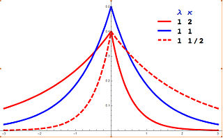
In probability theory and statistics, the asymmetric Laplace distribution (ALD) is a continuous probability distribution which is a generalization of the Laplace distribution. Just as the Laplace distribution consists of two exponential distributions of equal scale back-to-back about x = m, the asymmetric Laplace consists of two exponential distributions of unequal scale back to back about x = m, adjusted to assure continuity and normalization. The difference of two variates exponentially distributed with different means and rate parameters will be distributed according to the ALD. When the two rate parameters are equal, the difference will be distributed according to the Laplace distribution.

References

↑ Jaynes, Edwin T. (1968). "Prior Probabilities" (PDF). IEEE Transactions on Systems Science and Cybernetics. 4 (3): 227–241. doi:10.1109/TSSC.1968.300117. Archived (PDF) from the original on 2023-06-21. Retrieved 2023-06-30.
↑ Jaynes, Edwin T. (1973). "The Well-Posed Problem" (PDF). Foundations of Physics. 3 (4): 477–492. Bibcode:1973FoPh....3..477J. doi:10.1007/BF00709116. S2CID 2380040. Archived (PDF) from the original on 2023-06-22. Retrieved 2023-06-30.
↑ Jaynes, E. T. (1984). "Monkeys, Kangaroos, and N" (PDF). In Justice, James H. (ed.). Maximum Entropy and Bayesian Methods in Applied Statistics. Fourth Annual Workshop on Bayesian/Maximum Entropy Methods. Cambridge University Press. Retrieved 2023-11-13.
↑ Shackel, Nicholas (2007). "Bertrand's Paradox and the Principle of Indifference" (PDF). Philosophy of Science. 74 (2): 150–175. doi:10.1086/519028. JSTOR 519028. S2CID 15760612. Archived (PDF) from the original on 2022-01-28. Retrieved 2018-11-04.