Temperature dependence of viscosity

Last updated

Viscosity depends strongly on temperature. In liquids it usually decreases with increasing temperature, whereas, in most gases, viscosity increases with increasing temperature. This article discusses several models of this dependence, ranging from rigorous first-principles calculations for monatomic gases, to empirical correlations for liquids.

Contents

Understanding the temperature dependence of viscosity is important for many applications, for instance engineering lubricants that perform well under varying temperature conditions (such as in a car engine), since the performance of a lubricant depends in part on its viscosity. Engineering problems of this type fall under the purview of tribology.

Here dynamic viscosity is denoted by and kinematic viscosity by . The formulas given are valid only for an absolute temperature scale; therefore, unless stated otherwise temperatures are in kelvins.

Physical causes

Viscosity in gases arises from molecules traversing layers of flow and transferring momentum between layers. This transfer of momentum can be thought of as a frictional force between layers of flow. Since the momentum transfer is caused by free motion of gas molecules between collisions, increasing thermal agitation of the molecules results in a larger viscosity. Hence, gaseous viscosity increases with temperature.

In liquids, viscous forces are caused by molecules exerting attractive forces on each other across layers of flow. Increasing temperature results in a decrease in viscosity because a larger temperature means particles have greater thermal energy and are more easily able to overcome the attractive forces binding them together. An everyday example of this viscosity decrease is cooking oil moving more fluidly in a hot frying pan than in a cold one.

Gases

The kinetic theory of gases allows accurate calculation of the temperature-variation of gaseous viscosity. The theoretical basis of the kinetic theory is given by the Boltzmann equation and Chapman–Enskog theory, which allow accurate statistical modeling of molecular trajectories. In particular, given a model for intermolecular interactions, one can calculate with high precision the viscosity of monatomic and other simple gases (for more complex gases, such as those composed of polar molecules, additional assumptions must be introduced which reduce the accuracy of the theory). [1]

The viscosity predictions for four molecular models are discussed below. The predictions of the first three models (hard-sphere, power-law, and Sutherland) can be simply expressed in terms of elementary functions. The Lennard–Jones model predicts a more complicated -dependence, but is more accurate than the other three models and is widely used in engineering practice.

Hard-sphere kinetic theory

If one models gas molecules as elastic hard spheres (with mass and diameter ), then elementary kinetic theory predicts that viscosity increases with the square root of absolute temperature :

where is the Boltzmann constant. While correctly predicting the increase of gaseous viscosity with temperature, the trend is not accurate; the viscosity of real gases increases more rapidly than this. Capturing the actual dependence requires more realistic models of molecular interactions, in particular the inclusion of attractive interactions which are present in all real gases. [2]

Power-law force

A modest improvement over the hard-sphere model is a repulsive inverse power-law force, where the force between two molecules separated by distance is proportional to , where is an empirical parameter. [3] This is not a realistic model for real-world gases (except possibly at high temperature), but provides a simple illustration of how changing intermolecular interactions affects the predicted temperature dependence of viscosity. In this case, kinetic theory predicts an increase in temperature as , where . More precisely, if is the known viscosity at temperature , then

Taking recovers the hard-sphere result, . For finite , corresponding to softer repulsion, is greater than , which results in faster increase of viscosity compared with the hard-sphere model. Fitting to experimental data for hydrogen and helium gives predictions for and shown in the table. The model is modestly accurate for these two gases, but inaccurate for other gases.

Table: Inverse power law potential parameters for hydrogen and helium [3]
GasTemp. range (K)
Hydrogen 0.66812.9273–373
Helium 0.65713.743–1073

Sutherland model

Another simple model for gaseous viscosity is the Sutherland model, which adds weak intermolecular attractions to the hard-sphere model. [4] If the attractions are small, they can be treated perturbatively, which leads to

where , called the Sutherland constant, can be expressed in terms of the parameters of the intermolecular attractive force. Equivalently, if is a known viscosity at temperature , then

Values of obtained from fitting to experimental data are shown in the table below for several gases. The model is modestly accurate for a number of gases (nitrogen, oxygen, argon, air, and others), but inaccurate for other gases like hydrogen and helium. In general, it has been argued that the Sutherland model is actually a poor model of intermolecular interactions, and is useful only as a simple interpolation formula for a restricted set of gases over a restricted range of temperatures.

Table: Sutherland constants of selected gases [4]
Gas (K)Temp. range (K)
Dry air 113293–373
Helium 72.9293–373
Neon 64.1293–373
Argon 148293–373
Krypton 188289–373
Xenon 252288–373
Nitrogen 104.7293–1098
Oxygen 125288–1102

Lennard-Jones

Under fairly general conditions on the molecular model, the kinetic theory prediction for can be written in the form

where is called the collision integral and is a function of temperature as well as the parameters of the intermolecular interaction. [5] It is completely determined by the kinetic theory, being expressed in terms of integrals over collisional trajectories of pairs of molecules. In general, is a complicated function of both temperature and the molecular parameters; the power-law and Sutherland models are unusual in that can be expressed in terms of elementary functions.

The Lennard–Jones model assumes an intermolecular pair potential of the form

where and are parameters and is the distance separating the centers of mass of the molecules. As such, the model is designed for spherically symmetric molecules. Nevertheless, it is frequently used for non-spherically symmetric molecules provided these do not possess a large dipole moment. [5] [6]

The collisional integral for the Lennard-Jones model cannot be expressed exactly in terms of elementary functions. Nevertheless, it can be calculated numerically, and the agreement with experiment is good – not only for spherically symmetric molecules such as the noble gases, but also for many polyatomic gases as well. [6] An approximate form of has also been suggested: [7]

where . This equation has an average deviation of only 0.064 percent of the range .

Values of and estimated from experimental data are shown in the table below for several common gases.

Table: Lennard-Jones parameters of selected gases [8]
Gas (angstroms) (K)
Dry air 3.61797.0
Helium 2.57610.2
Hydrogen 2.91538.0
Argon 3.432122.4
Nitrogen 3.66799.8
Oxygen 3.433113
Carbon dioxide 3.996190
Methane 3.780154

Liquids

In contrast with gases, there is no systematic microscopic theory for liquid viscosity. [9] However, there are several empirical models which extrapolate a temperature dependence based on available experimental viscosities.

Two-parameter exponential

A simple and widespread empirical correlation for liquid viscosity is a two-parameter exponential:

This equation was first proposed in 1913, and is commonly known as the Andrade equation (named after British physicist Edward Andrade). It accurately describes many liquids over a range of temperatures. Its form can be motivated by modeling momentum transport at the molecular level as an activated rate process, [10] although the physical assumptions underlying such models have been called into question. [11]

The table below gives estimated values of and for representative liquids. Comprehensive tables of these parameters for hundreds of liquids can be found in the literature. [12]

Fitting parameters for the correlation [13]
LiquidChemical formulaA (mPa·s)B (K)Temp. range (K)
Bromine Br20.0445907.6269–302
Acetone C3H6O0.0177845.6193–333
Bromoform CHBr30.03321195278–363
Pentane C5H120.0191722.2143–313
Bromobenzene C6H5Br0.020881170273–423

Three- and four-parameter exponentials

One can also find tabulated exponentials with additional parameters, for example

and

Representative values are given in the tables below.

Fitting parameters for the correlation [14]
LiquidChemical formulaA (mPa·s)B (K)C (K−1)Temp. range (K)
Mercury Hg0.7754117.91124.04290–380
Fluorine F20.0906845.9739.37760–85
Lead Pb0.7610421.35266.85600–1200
Hydrazine N2H40.03625683.2983.603280–450
Octane C8H180.0078891456.2−51.44270–400
Fitting parameters for the correlation [13]
LiquidChemical formulaA (mPa·s)B (K)C (K−1)D (K−2)Temp. range (K)
Water H2O1.856·10−1142090.04527−3.376·10−5273–643
Ethanol C2H6O0.0020116140.00618−1.132·10−5168–516
Benzene C6H6100.69148.9−0.025442.222·10−5279–561
Cyclohexane C6H120.012301380−1.55·10−31.157·10−6280–553
Naphthalene C10H83.465·10−525170.01098−5.867·10−6354–748

Models for kinematic viscosity

The effect of temperature on the kinematic viscosity has also been described by a number of empirical equations. [15]

The Walther formula is typically written in the form

where is a shift constant, and and are empirical parameters. In lubricant specifications, normally only two temperatures are specified, in which case a standard value of = 0.7 is normally assumed.

The Wright model has the form

where an additional function , often a polynomial fit to experimental data, has been added to the Walther formula.

The Seeton model is based on curve fitting the viscosity dependence of many liquids (refrigerants, hydrocarbons and lubricants) versus temperature and applies over a large temperature and viscosity range:

where is absolute temperature in kelvins, is the kinematic viscosity in centistokes, is the zero order modified Bessel function of the second kind, and and are empirical parameters specific to each liquid.

For liquid metal viscosity as a function of temperature, Seeton proposed:

See also

Notes

  1. Chapman & Cowling (1970)
  2. Chapman & Cowling (1970), pp. 97–98, 226–230
  3. 1 2 Chapman & Cowling (1970), pp. 230–232
  4. 1 2 Chapman & Cowling (1970), pp. 232–234
  5. 1 2 Reid, Prausnitz, & Poling (1987), pp. 391–392
  6. 1 2 Bird, Stewart, & Lightfoot (2007), pp. 26–27
  7. Neufeld, Jansen, & Aziz (1972)
  8. Bird, Stewart, & Lightfoot (2007), pp. 864–865
  9. Reid, Prausnitz, & Poling (1987), p. 433
  10. Bird, Stewart, and Lightfoot (2007), pp. 29–31
  11. Hildebrand (1977)
  12. See Viswanath & Natarajan (1989); Viswanath et al (2007); Reid, Prausnitz, & Poling (1987); and references therein
  13. 1 2 Reid, Prausnitz, & Poling (1987)
  14. Viswanath & Natarajan (1989)
  15. Seeton (2006)

Related Research Articles

In a chemical reaction, chemical equilibrium is the state in which both the reactants and products are present in concentrations which have no further tendency to change with time, so that there is no observable change in the properties of the system. This state results when the forward reaction proceeds at the same rate as the reverse reaction. The reaction rates of the forward and backward reactions are generally not zero, but they are equal. Thus, there are no net changes in the concentrations of the reactants and products. Such a state is known as dynamic equilibrium.

<span class="mw-page-title-main">Normal distribution</span> Probability distribution

In statistics, a normal distribution or Gaussian distribution is a type of continuous probability distribution for a real-valued random variable. The general form of its probability density function is

In particle physics, the Dirac equation is a relativistic wave equation derived by British physicist Paul Dirac in 1928. In its free form, or including electromagnetic interactions, it describes all spin-12 massive particles, called "Dirac particles", such as electrons and quarks for which parity is a symmetry. It is consistent with both the principles of quantum mechanics and the theory of special relativity, and was the first theory to account fully for special relativity in the context of quantum mechanics. It was validated by accounting for the fine structure of the hydrogen spectrum in a completely rigorous way.

<span class="mw-page-title-main">Navier–Stokes equations</span> Equations describing the motion of viscous fluid substances

The Navier–Stokes equations are partial differential equations which describe the motion of viscous fluid substances, named after French engineer and physicist Claude-Louis Navier and Anglo-Irish physicist and mathematician George Gabriel Stokes. They were developed over several decades of progressively building the theories, from 1822 (Navier) to 1842-1850 (Stokes).

<span class="mw-page-title-main">Dynamo theory</span> Mechanism by which a celestial body generates a magnetic field

In physics, the dynamo theory proposes a mechanism by which a celestial body such as Earth or a star generates a magnetic field. The dynamo theory describes the process through which a rotating, convecting, and electrically conducting fluid can maintain a magnetic field over astronomical time scales. A dynamo is thought to be the source of the Earth's magnetic field and the magnetic fields of Mercury and the Jovian planets.

In physics, the Polyakov action is an action of the two-dimensional conformal field theory describing the worldsheet of a string in string theory. It was introduced by Stanley Deser and Bruno Zumino and independently by L. Brink, P. Di Vecchia and P. S. Howe in 1976, and has become associated with Alexander Polyakov after he made use of it in quantizing the string in 1981. The action reads:

Variational Bayesian methods are a family of techniques for approximating intractable integrals arising in Bayesian inference and machine learning. They are typically used in complex statistical models consisting of observed variables as well as unknown parameters and latent variables, with various sorts of relationships among the three types of random variables, as might be described by a graphical model. As typical in Bayesian inference, the parameters and latent variables are grouped together as "unobserved variables". Variational Bayesian methods are primarily used for two purposes:

  1. To provide an analytical approximation to the posterior probability of the unobserved variables, in order to do statistical inference over these variables.
  2. To derive a lower bound for the marginal likelihood of the observed data. This is typically used for performing model selection, the general idea being that a higher marginal likelihood for a given model indicates a better fit of the data by that model and hence a greater probability that the model in question was the one that generated the data.

In thermodynamics, an activity coefficient is a factor used to account for deviation of a mixture of chemical substances from ideal behaviour. In an ideal mixture, the microscopic interactions between each pair of chemical species are the same and, as a result, properties of the mixtures can be expressed directly in terms of simple concentrations or partial pressures of the substances present e.g. Raoult's law. Deviations from ideality are accommodated by modifying the concentration by an activity coefficient. Analogously, expressions involving gases can be adjusted for non-ideality by scaling partial pressures by a fugacity coefficient.

<span class="mw-page-title-main">Scaled inverse chi-squared distribution</span> Probability distribution

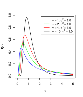
The scaled inverse chi-squared distribution is the distribution for x = 1/s2, where s2 is a sample mean of the squares of ν independent normal random variables that have mean 0 and inverse variance 1/σ2 = τ2. The distribution is therefore parametrised by the two quantities ν and τ2, referred to as the number of chi-squared degrees of freedom and the scaling parameter, respectively.

<span class="mw-page-title-main">Pearson distribution</span> Family of continuous probability distributions

The Pearson distribution is a family of continuous probability distributions. It was first published by Karl Pearson in 1895 and subsequently extended by him in 1901 and 1916 in a series of articles on biostatistics.

<span class="mw-page-title-main">Plasma parameters</span>

Plasma parameters define various characteristics of a plasma, an electrically conductive collection of charged particles that responds collectively to electromagnetic forces. Plasma typically takes the form of neutral gas-like clouds or charged ion beams, but may also include dust and grains. The behaviour of such particle systems can be studied statistically.

In statistics, stochastic volatility models are those in which the variance of a stochastic process is itself randomly distributed. They are used in the field of mathematical finance to evaluate derivative securities, such as options. The name derives from the models' treatment of the underlying security's volatility as a random process, governed by state variables such as the price level of the underlying security, the tendency of volatility to revert to some long-run mean value, and the variance of the volatility process itself, among others.

Collision frequency describes the rate of collisions between two atomic or molecular species in a given volume, per unit time. In an ideal gas, assuming that the species behave like hard spheres, the collision frequency between entities of species A and species B is:

<span class="mw-page-title-main">UNIFAC</span> Liquid equilibrium model in statistical thermodynamics

In statistical thermodynamics, the UNIFAC method is a semi-empirical system for the prediction of non-electrolyte activity in non-ideal mixtures. UNIFAC uses the functional groups present on the molecules that make up the liquid mixture to calculate activity coefficients. By using interactions for each of the functional groups present on the molecules, as well as some binary interaction coefficients, the activity of each of the solutions can be calculated. This information can be used to obtain information on liquid equilibria, which is useful in many thermodynamic calculations, such as chemical reactor design, and distillation calculations.

<span class="mw-page-title-main">Viscosity</span> Resistance of a fluid to shear deformation

The viscosity of a fluid is a measure of its resistance to deformation at a given rate. For liquids, it corresponds to the informal concept of "thickness": for example, syrup has a higher viscosity than water.

Chapman–Enskog theory provides a framework in which equations of hydrodynamics for a gas can be derived from the Boltzmann equation. The technique justifies the otherwise phenomenological constitutive relations appearing in hydrodynamical descriptions such as the Navier–Stokes equations. In doing so, expressions for various transport coefficients such as thermal conductivity and viscosity are obtained in terms of molecular parameters. Thus, Chapman–Enskog theory constitutes an important step in the passage from a microscopic, particle-based description to a continuum hydrodynamical one.

In statistics and probability theory, the nonparametric skew is a statistic occasionally used with random variables that take real values. It is a measure of the skewness of a random variable's distribution—that is, the distribution's tendency to "lean" to one side or the other of the mean. Its calculation does not require any knowledge of the form of the underlying distribution—hence the name nonparametric. It has some desirable properties: it is zero for any symmetric distribution; it is unaffected by a scale shift; and it reveals either left- or right-skewness equally well. In some statistical samples it has been shown to be less powerful than the usual measures of skewness in detecting departures of the population from normality.

In statistics, the variance function is a smooth function which depicts the variance of a random quantity as a function of its mean. The variance function is a measure of heteroscedasticity and plays a large role in many settings of statistical modelling. It is a main ingredient in the generalized linear model framework and a tool used in non-parametric regression, semiparametric regression and functional data analysis. In parametric modeling, variance functions take on a parametric form and explicitly describe the relationship between the variance and the mean of a random quantity. In a non-parametric setting, the variance function is assumed to be a smooth function.

The shear viscosity of a fluid is a material property that describes the friction between internal neighboring fluid surfaces flowing with different fluid velocities. This friction is the effect of (linear) momentum exchange caused by molecules with sufficient energy to move between these fluid sheets due to fluctuations in their motion. The viscosity is not a material constant, but a material property that depends on temperature, pressure, fluid mixture composition, local velocity variations. This functional relationship is described by a mathematical viscosity model called a constitutive equation which is usually far more complex than the defining equation of shear viscosity. One such complicating feature is the relation between the viscosity model for a pure fluid and the model for a fluid mixture which is called mixing rules. When scientists and engineers use new arguments or theories to develop a new viscosity model, instead of improving the reigning model, it may lead to the first model in a new class of models. This article will display one or two representative models for different classes of viscosity models, and these classes are:

In probability theory, a log-t distribution or log-Student t distribution is a probability distribution of a random variable whose logarithm is distributed in accordance with a Student's t-distribution. If X is a random variable with a Student's t-distribution, then Y = exp(X) has a log-t distribution; likewise, if Y has a log-t distribution, then X = log(Y) has a Student's t-distribution.

References