In numerical analysis, the Crank–Nicolson method is a finite difference method used for numerically solving the heat equation and similar partial differential equations. It is a second-order method in time. It is implicit in time, can be written as an implicit Runge–Kutta method, and it is numerically stable. The method was developed by John Crank and Phyllis Nicolson in the mid 20th century.
In mathematics, the convergence condition by Courant–Friedrichs–Lewy is a necessary condition for convergence while solving certain partial differential equations numerically. It arises in the numerical analysis of explicit time integration schemes, when these are used for the numerical solution. As a consequence, the time step must be less than a certain upper bound, given a fixed spatial increment, in many explicit time-marching computer simulations; otherwise, the simulation produces incorrect or unstable results. The condition is named after Richard Courant, Kurt Friedrichs, and Hans Lewy who described it in their 1928 paper.
An eikonal equation is a non-linear first-order partial differential equation that is encountered in problems of wave propagation.
In numerical methods, total variation diminishing (TVD) is a property of certain discretization schemes used to solve hyperbolic partial differential equations. The most notable application of this method is in computational fluid dynamics. The concept of TVD was introduced by Ami Harten.
In numerical analysis and computational fluid dynamics, Godunov's scheme is a conservative numerical scheme, suggested by Sergei Godunov in 1959, for solving partial differential equations. One can think of this method as a conservative finite volume method which solves exact, or approximate Riemann problems at each inter-cell boundary. In its basic form, Godunov's method is first order accurate in both space and time, yet can be used as a base scheme for developing higher-order methods.
In the study of partial differential equations, the MUSCL scheme is a finite volume method that can provide highly accurate numerical solutions for a given system, even in cases where the solutions exhibit shocks, discontinuities, or large gradients. MUSCL stands for Monotonic Upstream-centered Scheme for Conservation Laws, and the term was introduced in a seminal paper by Bram van Leer. In this paper he constructed the first high-order, total variation diminishing (TVD) scheme where he obtained second order spatial accuracy.

The Navier–Stokes existence and smoothness problem concerns the mathematical properties of solutions to the Navier–Stokes equations, a system of partial differential equations that describe the motion of a fluid in space. Solutions to the Navier–Stokes equations are used in many practical applications. However, theoretical understanding of the solutions to these equations is incomplete. In particular, solutions of the Navier–Stokes equations often include turbulence, which remains one of the greatest unsolved problems in physics, despite its immense importance in science and engineering.
In numerical analysis, finite-difference methods (FDM) are a class of numerical techniques for solving differential equations by approximating derivatives with finite differences. Both the spatial domain and time domain are discretized, or broken into a finite number of intervals, and the values of the solution at the end points of the intervals are approximated by solving algebraic equations containing finite differences and values from nearby points.
The Lax–Wendroff method, named after Peter Lax and Burton Wendroff, is a numerical method for the solution of hyperbolic partial differential equations, based on finite differences. It is second-order accurate in both space and time. This method is an example of explicit time integration where the function that defines the governing equation is evaluated at the current time.
In applied mathematics, discontinuous Galerkin methods (DG methods) form a class of numerical methods for solving differential equations. They combine features of the finite element and the finite volume framework and have been successfully applied to hyperbolic, elliptic, parabolic and mixed form problems arising from a wide range of applications. DG methods have in particular received considerable interest for problems with a dominant first-order part, e.g. in electrodynamics, fluid mechanics and plasma physics.
In computational fluid dynamics, the MacCormack method is a widely used discretization scheme for the numerical solution of hyperbolic partial differential equations. This second-order finite difference method was introduced by Robert W. MacCormack in 1969. The MacCormack method is elegant and easy to understand and program.
Nonstandard finite difference schemes is a general set of methods in numerical analysis that gives numerical solutions to differential equations by constructing a discrete model. The general rules for such schemes are not precisely known.
The Lax–Friedrichs method, named after Peter Lax and Kurt O. Friedrichs, is a numerical method for the solution of hyperbolic partial differential equations based on finite differences. The method can be described as the FTCS scheme with a numerical dissipation term of 1/2. One can view the Lax–Friedrichs method as an alternative to Godunov's scheme, where one avoids solving a Riemann problem at each cell interface, at the expense of adding artificial viscosity.
In numerical analysis, the FTCS method is a finite difference method used for numerically solving the heat equation and similar parabolic partial differential equations. It is a first-order method in time, explicit in time, and is conditionally stable when applied to the heat equation. When used as a method for advection equations, or more generally hyperbolic partial differential equations, it is unstable unless artificial viscosity is included. The abbreviation FTCS was first used by Patrick Roache.
In numerical analysis, von Neumann stability analysis is a procedure used to check the stability of finite difference schemes as applied to linear partial differential equations. The analysis is based on the Fourier decomposition of numerical error and was developed at Los Alamos National Laboratory after having been briefly described in a 1947 article by British researchers Crank and Nicolson. This method is an example of explicit time integration where the function that defines governing equation is evaluated at the current time. Later, the method was given a more rigorous treatment in an article co-authored by John von Neumann.
The hybrid difference scheme is a method used in the numerical solution for convection–diffusion problems. It was introduced by Spalding (1970). It is a combination of central difference scheme and upwind difference scheme as it exploits the favorable properties of both of these schemes.
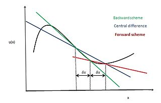
In applied mathematics, the central differencing scheme is a finite difference method that optimizes the approximation for the differential operator in the central node of the considered patch and provides numerical solutions to differential equations. It is one of the schemes used to solve the integrated convection–diffusion equation and to calculate the transported property Φ at the e and w faces, where e and w are short for east and west. The method's advantages are that it is easy to understand and implement, at least for simple material relations; and that its convergence rate is faster than some other finite differencing methods, such as forward and backward differencing. The right side of the convection-diffusion equation, which basically highlights the diffusion terms, can be represented using central difference approximation. To simplify the solution and analysis, linear interpolation can be used logically to compute the cell face values for the left side of this equation, which is nothing but the convective terms. Therefore, cell face values of property for a uniform grid can be written as:
Unsteady flows are characterized as flows in which the properties of the fluid are time dependent. It gets reflected in the governing equations as the time derivative of the properties are absent. For Studying Finite-volume method for unsteady flow there is some governing equations >
The convection–diffusion equation describes the flow of heat, particles, or other physical quantities in situations where there is both diffusion and convection or advection. For information about the equation, its derivation, and its conceptual importance and consequences, see the main article convection–diffusion equation. This article describes how to use a computer to calculate an approximate numerical solution of the discretized equation, in a time-dependent situation.
In numerical mathematics, Beam and Warming scheme or Beam–Warming implicit scheme introduced in 1978 by Richard M. Beam and R. F. Warming, is a second order accurate implicit scheme, mainly used for solving non-linear hyperbolic equations. It is not used much nowadays.


