Directional Cubic Convolution Interpolation

Last updated

Directional Cubic Convolution Interpolation (DCCI) is an edge-directed image scaling algorithm created by Dengwen Zhou and Xiaoliu Shen. [1]

Contents

By taking into account the edges in an image, this scaling algorithm reduces artifacts common to other image scaling algorithms. For example, staircase artifacts on diagonal lines and curves are eliminated.

The algorithm resizes an image to 2x its original dimensions, minus 1. [2]

The algorithm

The algorithm works in three main steps:

  1. Copy the original pixels to the output image, with gaps between the pixels.
  2. Calculate the pixels for the diagonal gaps.
  3. Calculate the pixels for the remaining horizontal and vertical gaps.

DCCI interpolation pixel grid layout.svg

Calculating pixels in diagonal gaps

Evaluation of diagonal pixels is done on the original image data in a 4×4 region, with the new pixel that is being calculated in the center, in the gap between the original pixels. This can also be thought of as the 7×7 region in the enlarged image centered on the new pixel to calculate, and the original pixels have already been copied.

The algorithm decides one of three cases:

Calculating diagonal edge strength

Let d1 be the sum of edges in the up-right direction, and d2 be the sum of edges in the down-right direction.

To calculate d1, take the sum of abs(P(X, Y) - P(X - 1, Y + 1)), in the region of X = 1 to 3, and Y = 0 to 2.

To calculate d2, take the sum of abs(P(X, Y) - P(X + 1, Y + 1)), in the region of X = 0 to 2, and Y = 0 to 2.

DCCI interpolation diagonal pixels 01.svg

Interpolating pixels

If (1 + d1) / (1 + d2) > 1.15, then there is an edge in the up-right direction. If (1 + d2) / (1 + d1) > 1.15, then there is an edge in the down-right direction.

Otherwise, one is in a smooth area. To avoid division and floating-point operations, this can also be expressed as 100 * (1 + d1) > 115 * (1 + d2), and 100 * (1 + d2) > 115 * (1 + d1).

Up-right edge

For an edge in the up-right direction, one interpolates in the down-right direction.

Output pixel = (-1 * P(0, 0) + 9 * P(1, 1) + 9 * P(2, 2) - 1 * P(3, 3)) / 16

The pixel value will need to be forced to the valid range of pixel values (usually 0 to 255).

Down-right edge

For an edge in the down-right direction, one interpolates in the up-right direction.

Output pixel = (-1 * P(3, 0) + 9 * P(2, 1) + 9 * P(1, 2) - 1 * P(0, 3)) / 16

The pixel value will need to be forced to the valid range of pixel values (usually 0 to 255).

Smooth area

In the smooth area, edge strength from up-right will contribute to the down-right sampled pixel, and edge strength from down-right will contribute to the up-right sampled pixel.

w1 = 1 / (1 + d1 ^ 5)

w2 = 1 / (1 + d2 ^ 5)

weight1 = w1 / (w1 + w2)

weight2 = w2 / (w1 + w2)

DownRightPixel = (-1 * P(0, 0) + 9 * P(1, 1) + 9 * P(2, 2) - 1 * P(3, 3)) / 16

UpRightPixel = (-1 * P(3, 0) + 9 * P(2, 1) + 9 * P(1, 2) - 1 * P(0, 3)) / 16

Output Pixel = DownRightPixel * weight1 + UpRightPixel * weight2

The pixel value will need to be forced to the valid range of pixel values (usually 0 to 255).

Calculating remaining pixels

Evaluating the remaining pixels is done on the scaled image data in a 7×7 region, with the new pixel that is being calculated in the center. These calculations either depend on the original pixels of the image or on a diagonal pixel calculated in the previous step.

The algorithm decides one of three cases:

Calculating horizontal/vertical edge strength

Let d1 be the sum of edges in the horizontal direction, and d2 be the sum of edges in the vertical direction.

Consider a 7×7 diamond-shaped region centered on the pixel to calculate, using only pixel values from the original, and pixel values added from the diagonal direction.

To calculate d1, take the sum of the absolute differences of the horizontal edges, sampling these pixel values:

| P(X+1, Y-2) - P(X-1, Y-2) | + | P(X+2, Y-1) - P(X, Y-1) | + | P(X, Y-1) - P(X-2, Y-1) | + | P(X+3, Y) - P(X+1, Y) | + | P(X+1, Y) - P(X-1, Y) | + | P(X-1, Y) - P(X-3, Y) | + | P(X+2, Y+1) - P(X, Y+1) | + | P(X, Y+1) - P(X-2, Y+1) | + | P(X+1, Y+2) - P(X-1, Y+2) | 

To calculate d2, take the sum of the absolute differences of the vertical edges, sampling these pixel values:

| P(X-2, Y+1) - P(X-2, Y-1) | + | P(X-1, Y+2) - P(X-1, Y) | + | P(X-1, Y) - P(X-1, Y-2) | + | P(X, Y+3) - P(X, Y+1) | + | P(X, Y+1) - P(X, Y-1) | + | P(X, Y-1) - P(X, Y-3) | + | P(X+1, Y+2) - P(X+1, Y) | + | P(X+1, Y) - P(X+1, Y-2) | + | P(X+2, Y+1) - P(X+2, Y-1) | 

DCCI interpolation remaining pixels 01.svg

Interpolating pixels

If (1 + d1) / (1 + d2) > 1.15, then one has an edge in the horizontal direction.

If (1 + d2) / (1 + d1) > 1.15, then one has an edge in the vertical direction.

Otherwise, one is in the smooth area.

To avoid division floating-point operations, this can also be expressed as 100 * (1 + d1) > 115 * (1 + d2), and 100 * (1 + d2) > 115 * (1 + d1).

Horizontal edge

For a horizontal edge, one interpolates in the vertical direction, using only the column centered at the pixel.

Output pixel = (-1 * P(X, Y - 3) + 9 * P(X, Y - 1) + 9 * P(X, Y + 1) - 1 * P(X, Y + 3)) / 16

The pixel value will need to be forced to the valid range of pixel values (usually 0 to 255).

Vertical edge

For a vertical edge, one interpolates in the horizontal direction, using only the row centered at the pixel.

Output pixel = (-1 * P(X - 3, Y) + 9 * P(X - 1, Y) + 9 * P(X + 1, Y) - 1 * P(X + 3, Y)) / 16

The pixel value will need to be forced to the valid range of pixel values (usually 0 to 255).

Smooth area

In the smooth area, horizontal edge strength will contribute to the weight for the vertically sampled pixel, and vertical edge strength will contribute to the weight for the horizontally sampled pixel.

w1 = 1 / (1 + d1 ^ 5)

w2 = 1 / (1 + d2 ^ 5)

weight1 = w1 / (w1 + w2)

weight2 = w2 / (w1 + w2)

HorizontalPixel = (-1 * P(X - 3, Y) + 9 * P(X - 1, Y) + 9 * P(X + 1, Y) - 1 * P(X + 3, Y)) / 16

VerticalPixel = (-1 * P(X, Y - 3) + 9 * P(X, Y - 1) + 9 * P(X, Y + 1) - 1 * P(X, Y + 3)) / 16

Output Pixel = VerticalPixel * weight1 + HorizontalPixel * weight2

The pixel value will need to be forced to the valid range of pixel values (usually 0 to 255).

Not specified

Boundary pixels

The algorithm does not define what to do when sampling boundary areas outside of the image. Possible things to do include replicating the boundary pixel, wrapping pixels from the other side of the image, wrapping the same side of the image in reverse, or using a particular border color value.

Color images

Color images are not specified by the algorithm, however, one can sum all RGB component differences when calculating edge strength, and use all RGB components when interpolating the pixels. Or one could split to YCbCr, process only the luma component and stretch the chroma using a different algorithm.

See also

Related Research Articles

In digital signal processing, spatial anti-aliasing is a technique for minimizing the distortion artifacts known as aliasing when representing a high-resolution image at a lower resolution. Anti-aliasing is used in digital photography, computer graphics, digital audio, and many other applications.

Texture mapping

Texture mapping is a method for defining high frequency detail, surface texture, or color information on a computer-generated graphic or 3D model. The original technique was pioneered by Edwin Catmull in 1974.

Shading Depicting depth through varying levels of darkness

Shading refers to the depiction of depth perception in 3D models or illustrations by varying the level of darkness. Shading tries to approximate local behavior of light on the object's surface and is not to be confused with techniques of adding shadows, such as shadow mapping or shadow volumes, which fall under global behavior of light.

Sobel operator

The Sobel operator, sometimes called the Sobel–Feldman operator or Sobel filter, is used in image processing and computer vision, particularly within edge detection algorithms where it creates an image emphasising edges. It is named after Irwin Sobel and Gary Feldman, colleagues at the Stanford Artificial Intelligence Laboratory (SAIL). Sobel and Feldman presented the idea of an "Isotropic 3x3 Image Gradient Operator" at a talk at SAIL in 1968. Technically, it is a discrete differentiation operator, computing an approximation of the gradient of the image intensity function. At each point in the image, the result of the Sobel–Feldman operator is either the corresponding gradient vector or the norm of this vector. The Sobel–Feldman operator is based on convolving the image with a small, separable, and integer-valued filter in the horizontal and vertical directions and is therefore relatively inexpensive in terms of computations. On the other hand, the gradient approximation that it produces is relatively crude, in particular for high-frequency variations in the image.

Canny edge detector

The Canny edge detector is an edge detection operator that uses a multi-stage algorithm to detect a wide range of edges in images. It was developed by John F. Canny in 1986. Canny also produced a computational theory of edge detection explaining why the technique works.

Bayer filter Color filter array

A Bayer filter mosaic is a color filter array (CFA) for arranging RGB color filters on a square grid of photosensors. Its particular arrangement of color filters is used in most single-chip digital image sensors used in digital cameras, camcorders, and scanners to create a color image. The filter pattern is half green, one quarter red and one quarter blue, hence is also called BGGR,RGBG, GRBG, or RGGB.

Bilinear interpolation

In mathematics, bilinear interpolation is an extension of linear interpolation for interpolating functions of two variables on a rectilinear 2D grid.

Bicubic interpolation

In mathematics, bicubic interpolation is an extension of cubic interpolation for interpolating data points on a two-dimensional regular grid. The interpolated surface is smoother than corresponding surfaces obtained by bilinear interpolation or nearest-neighbor interpolation. Bicubic interpolation can be accomplished using either Lagrange polynomials, cubic splines, or cubic convolution algorithm.

Inverse distance weighting (IDW) is a type of deterministic method for multivariate interpolation with a known scattered set of points. The assigned values to unknown points are calculated with a weighted average of the values available at the known points.

Pixel-art scaling algorithms

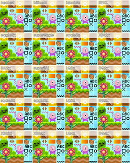
Pixel-art scaling algorithms are graphical filters that are often used in video game console emulators to enhance hand-drawn 2D pixel art graphics. The re-scaling of pixel art is a specialist sub-field of image rescaling.

Gaussian blur

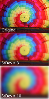
In image processing, a Gaussian blur is the result of blurring an image by a Gaussian function.

Lanczos resampling

Lanczos filtering and Lanczos resampling are two applications of a mathematical formula. It can be used as a low-pass filter or used to smoothly interpolate the value of a digital signal between its samples. In the latter case it maps each sample of the given signal to a translated and scaled copy of the Lanczos kernel, which is a sinc function windowed by the central lobe of a second, longer, sinc function. The sum of these translated and scaled kernels is then evaluated at the desired points.

Image scaling Changing the resolution of a digital image

In computer graphics and digital imaging, imagescaling refers to the resizing of a digital image. In video technology, the magnification of digital material is known as upscaling or resolution enhancement.

Marching squares is a computer graphics algorithm that generates contours for a two-dimensional scalar field. A similar method can be used to contour 2D triangle meshes.

Image gradient

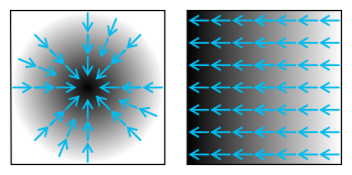
An image gradient is a directional change in the intensity or color in an image. The gradient of the image is one of the fundamental building blocks in image processing. For example, the Canny edge detector uses image gradient for edge detection. In graphics software for digital image editing, the term gradient or color gradient is also used for a gradual blend of color which can be considered as an even gradation from low to high values, as used from white to black in the images to the right. Another name for this is color progression.

A box blur is a spatial domain linear filter in which each pixel in the resulting image has a value equal to the average value of its neighboring pixels in the input image. It is a form of low-pass ("blurring") filter. A 3 by 3 box blur can be written as matrix

In computer vision, speeded up robust features (SURF) is a patented local feature detector and descriptor. It can be used for tasks such as object recognition, image registration, classification, or 3D reconstruction. It is partly inspired by the scale-invariant feature transform (SIFT) descriptor. The standard version of SURF is several times faster than SIFT and claimed by its authors to be more robust against different image transformations than SIFT.

In image processing, a kernel, convolution matrix, or mask is a small matrix. It is used for blurring, sharpening, embossing, edge detection, and more. This is accomplished by doing a convolution between a kernel and an image.

In image processing, line detection is an algorithm that takes a collection of n edge points and finds all the lines on which these edge points lie. The most popular line detectors are the Hough transform and convolution-based techniques.

Semi-global matching (SGM) is a computer vision algorithm for the estimation of a dense disparity map from a rectified stereo image pair, introduced in 2005 by Heiko Hirschmüller while working at the German Aerospace Center. Given its predictable run time, its favourable trade-off between quality of the results and computing time, and its suitability for fast parallel implementation in ASIC or FPGA, it has encountered wide adoption in real-time stereo vision applications such as robotics and advanced driver assistance systems.

References

  1. Dengwen Zhou; Xiaoliu Shen. "Image Zooming Using Directional Cubic Convolution Interpolation" . Retrieved 13 September 2015.
  2. Sabir, Essaïd; Medromi, Hicham; Sadik, Mohamed (2016-02-02). Advances in Ubiquitous Networking: Proceedings of the UNet'15. Springer. ISBN   978-981-287-990-5.