The Fresnel equations describe the reflection and transmission of light when incident on an interface between different optical media. They were deduced by French engineer and physicist Augustin-Jean Fresnel who was the first to understand that light is a transverse wave, when no one realized that the waves were electric and magnetic fields. For the first time, polarization could be understood quantitatively, as Fresnel's equations correctly predicted the differing behaviour of waves of the s and p polarizations incident upon a material interface.
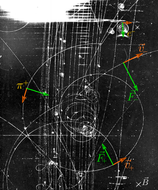
In physics, specifically in electromagnetism, the Lorentz force is the combination of electric and magnetic force on a point charge due to electromagnetic fields. A particle of charge q moving with a velocity v in an electric field E and a magnetic field B experiences a force of
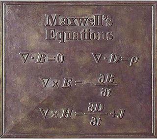
Maxwell's equations, or Maxwell–Heaviside equations, are a set of coupled partial differential equations that, together with the Lorentz force law, form the foundation of classical electromagnetism, classical optics, electric and magnetic circuits. The equations provide a mathematical model for electric, optical, and radio technologies, such as power generation, electric motors, wireless communication, lenses, radar, etc. They describe how electric and magnetic fields are generated by charges, currents, and changes of the fields. The equations are named after the physicist and mathematician James Clerk Maxwell, who, in 1861 and 1862, published an early form of the equations that included the Lorentz force law. Maxwell first used the equations to propose that light is an electromagnetic phenomenon. The modern form of the equations in their most common formulation is credited to Oliver Heaviside.
In physics, the Poynting vector represents the directional energy flux or power flow of an electromagnetic field. The SI unit of the Poynting vector is the watt per square metre (W/m2); kg/s3 in base SI units. It is named after its discoverer John Henry Poynting who first derived it in 1884. Nikolay Umov is also credited with formulating the concept. Oliver Heaviside also discovered it independently in the more general form that recognises the freedom of adding the curl of an arbitrary vector field to the definition. The Poynting vector is used throughout electromagnetics in conjunction with Poynting's theorem, the continuity equation expressing conservation of electromagnetic energy, to calculate the power flow in electromagnetic fields.

Inductance is the tendency of an electrical conductor to oppose a change in the electric current flowing through it. The electric current produces a magnetic field around the conductor. The magnetic field strength depends on the magnitude of the electric current, and follows any changes in the magnitude of the current. From Faraday's law of induction, any change in magnetic field through a circuit induces an electromotive force (EMF) (voltage) in the conductors, a process known as electromagnetic induction. This induced voltage created by the changing current has the effect of opposing the change in current. This is stated by Lenz's law, and the voltage is called back EMF.

Johnson–Nyquist noise is the electronic noise generated by the thermal agitation of the charge carriers inside an electrical conductor at equilibrium, which happens regardless of any applied voltage. Thermal noise is present in all electrical circuits, and in sensitive electronic equipment can drown out weak signals, and can be the limiting factor on sensitivity of electrical measuring instruments. Thermal noise increases with temperature. Some sensitive electronic equipment such as radio telescope receivers are cooled to cryogenic temperatures to reduce thermal noise in their circuits. The generic, statistical physical derivation of this noise is called the fluctuation-dissipation theorem, where generalized impedance or generalized susceptibility is used to characterize the medium.
In classical electromagnetism, Ampère's circuital law relates the circulation of a magnetic field around a closed loop to the electric current passing through the loop.
Acoustic impedance and specific acoustic impedance are measures of the opposition that a system presents to the acoustic flow resulting from an acoustic pressure applied to the system. The SI unit of acoustic impedance is the pascal-second per cubic metre, or in the MKS system the rayl per square metre (Rayl/m2), while that of specific acoustic impedance is the pascal-second per metre (Pa·s/m), or in the MKS system the rayl (Rayl). There is a close analogy with electrical impedance, which measures the opposition that a system presents to the electric current resulting from a voltage applied to the system.

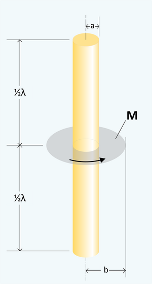
In electromagnetism, the magnetic moment or magnetic dipole moment is the combination of strength and orientation of a magnet or other object or system that exerts a magnetic field. The magnetic dipole moment of an object determines the magnitude of torque the object experiences in a given magnetic field. When the same magnetic field is applied, objects with larger magnetic moments experience larger torques. The strength of this torque depends not only on the magnitude of the magnetic moment but also on its orientation relative to the direction of the magnetic field. Its direction points from the south pole to north pole of the magnet.
In electromagnetism, displacement current density is the quantity ∂D/∂t appearing in Maxwell's equations that is defined in terms of the rate of change of D, the electric displacement field. Displacement current density has the same units as electric current density, and it is a source of the magnetic field just as actual current is. However it is not an electric current of moving charges, but a time-varying electric field. In physical materials, there is also a contribution from the slight motion of charges bound in atoms, called dielectric polarization.
In classical electromagnetism, polarization density is the vector field that expresses the volumetric density of permanent or induced electric dipole moments in a dielectric material. When a dielectric is placed in an external electric field, its molecules gain electric dipole moment and the dielectric is said to be polarized.
The Vlasov equation is a differential equation describing time evolution of the distribution function of plasma consisting of charged particles with long-range interaction, such as the Coulomb interaction. The equation was first suggested for the description of plasma by Anatoly Vlasov in 1938 and later discussed by him in detail in a monograph.
In classical electromagnetism, reciprocity refers to a variety of related theorems involving the interchange of time-harmonic electric current densities (sources) and the resulting electromagnetic fields in Maxwell's equations for time-invariant linear media under certain constraints. Reciprocity is closely related to the concept of symmetric operators from linear algebra, applied to electromagnetism.
The electromagnetic wave equation is a second-order partial differential equation that describes the propagation of electromagnetic waves through a medium or in a vacuum. It is a three-dimensional form of the wave equation. The homogeneous form of the equation, written in terms of either the electric field E or the magnetic field B, takes the form:
The telegrapher's equations are a set of two coupled, linear equations that predict the voltage and current distributions on a linear electrical transmission line. The equations are important because they allow transmission lines to be analyzed using circuit theory. The equations and their solutions are applicable from 0 Hz to frequencies at which the transmission line structure can support higher order non-TEM modes. The equations can be expressed in both the time domain and the frequency domain. In the time domain the independent variables are distance and time. The resulting time domain equations are partial differential equations of both time and distance. In the frequency domain the independent variables are distance and either frequency, or complex frequency, The frequency domain variables can be taken as the Laplace transform or Fourier transform of the time domain variables or they can be taken to be phasors. The resulting frequency domain equations are ordinary differential equations of distance. An advantage of the frequency domain approach is that differential operators in the time domain become algebraic operations in frequency domain.
In electrical engineering, dielectric loss quantifies a dielectric material's inherent dissipation of electromagnetic energy. It can be parameterized in terms of either the loss angleδ or the corresponding loss tangenttan(δ). Both refer to the phasor in the complex plane whose real and imaginary parts are the resistive (lossy) component of an electromagnetic field and its reactive (lossless) counterpart.
There are various mathematical descriptions of the electromagnetic field that are used in the study of electromagnetism, one of the four fundamental interactions of nature. In this article, several approaches are discussed, although the equations are in terms of electric and magnetic fields, potentials, and charges with currents, generally speaking.
When an electromagnetic wave travels through a medium in which it gets attenuated, it undergoes exponential decay as described by the Beer–Lambert law. However, there are many possible ways to characterize the wave and how quickly it is attenuated. This article describes the mathematical relationships among:

The gyrator–capacitor model - sometimes also the capacitor-permeance model - is a lumped-element model for magnetic circuits, that can be used in place of the more common resistance–reluctance model. The model makes permeance elements analogous to electrical capacitance rather than electrical resistance. Windings are represented as gyrators, interfacing between the electrical circuit and the magnetic model.
Heat transfer physics describes the kinetics of energy storage, transport, and energy transformation by principal energy carriers: phonons, electrons, fluid particles, and photons. Heat is thermal energy stored in temperature-dependent motion of particles including electrons, atomic nuclei, individual atoms, and molecules. Heat is transferred to and from matter by the principal energy carriers. The state of energy stored within matter, or transported by the carriers, is described by a combination of classical and quantum statistical mechanics. The energy is different made (converted) among various carriers. The heat transfer processes are governed by the rates at which various related physical phenomena occur, such as the rate of particle collisions in classical mechanics. These various states and kinetics determine the heat transfer, i.e., the net rate of energy storage or transport. Governing these process from the atomic level to macroscale are the laws of thermodynamics, including conservation of energy.