Mathematical descriptions of the electromagnetic field

Last updated

There are various mathematical descriptions of the electromagnetic field that are used in the study of electromagnetism, one of the four fundamental interactions of nature. In this article, several approaches are discussed, although the equations are in terms of electric and magnetic fields, potentials, and charges with currents, generally speaking.

Contents

Vector field approach

The most common description of the electromagnetic field uses two three-dimensional vector fields called the electric field and the magnetic field. These vector fields each have a value defined at every point of space and time and are thus often regarded as functions of the space and time coordinates. As such, they are often written as E(x, y, z, t) (electric field) and B(x, y, z, t) (magnetic field).

If only the electric field (E) is non-zero, and is constant in time, the field is said to be an electrostatic field. Similarly, if only the magnetic field (B) is non-zero and is constant in time, the field is said to be a magnetostatic field. However, if either the electric or magnetic field has a time-dependence, then both fields must be considered together as a coupled electromagnetic field using Maxwell's equations.

Maxwell's equations in the vector field approach

The behaviour of electric and magnetic fields, whether in cases of electrostatics, magnetostatics, or electrodynamics (electromagnetic fields), is governed by Maxwell-Heaviside's equations:

Maxwell's equations ( vector fields )
   Gauss's law
   Gauss's law for magnetism
   Faraday's law of induction
   Ampère-Maxwell law

where ρ is the charge density, which can (and often does) depend on time and position, ε0 is the electric constant, μ0 is the magnetic constant, and J is the current per unit area, also a function of time and position. The equations take this form with the International System of Quantities.

When dealing with only nondispersive isotropic linear materials, Maxwell's equations are often modified to ignore bound charges by replacing the permeability and permittivity of free space with the permeability and permittivity of the linear material in question. For some materials that have more complex responses to electromagnetic fields, these properties can be represented by tensors, with time-dependence related to the material's ability to respond to rapid field changes (dispersion (optics), Green–Kubo relations), and possibly also field dependencies representing nonlinear and/or nonlocal material responses to large amplitude fields (nonlinear optics).

Potential field approach

Many times in the use and calculation of electric and magnetic fields, the approach used first computes an associated potential: the electric potential, , for the electric field, and the magnetic vector potential, A, for the magnetic field. The electric potential is a scalar field, while the magnetic potential is a vector field. This is why sometimes the electric potential is called the scalar potential and the magnetic potential is called the vector potential. These potentials can be used to find their associated fields as follows:

Maxwell's equations in potential formulation

These relations can be substituted into Maxwell's equations to express the latter in terms of the potentials. Faraday's law and Gauss's law for magnetism (the homogeneous equations) turn out to be identically true for any potentials. This is because of the way the fields are expressed as gradients and curls of the scalar and vector potentials. The homogeneous equations in terms of these potentials involve the divergence of the curl and the curl of the gradient , which are always zero. The other two of Maxwell's equations (the inhomogeneous equations) are the ones that describe the dynamics in the potential formulation.

Maxwell's equations (potential formulation)

These equations taken together are as powerful and complete as Maxwell's equations. Moreover, the problem has been reduced somewhat, as the electric and magnetic fields together had six components to solve for. [1] In the potential formulation, there are only four components: the electric potential and the three components of the vector potential. However, the equations are messier than Maxwell's equations using the electric and magnetic fields.

Gauge freedom

These equations can be simplified by taking advantage of the fact that the electric and magnetic fields are physically meaningful quantities that can be measured; the potentials are not. There is a freedom to constrain the form of the potentials provided that this does not affect the resultant electric and magnetic fields, called gauge freedom. Specifically for these equations, for any choice of a twice-differentiable scalar function of position and time λ, if (φ, A) is a solution for a given system, then so is another potential (φ′, A′) given by:

This freedom can be used to simplify the potential formulation. Either of two such scalar functions is typically chosen: the Coulomb gauge and the Lorenz gauge.

Coulomb gauge

The Coulomb gauge is chosen in such a way that , which corresponds to the case of magnetostatics. In terms of λ, this means that it must satisfy the equation

This choice of function results in the following formulation of Maxwell's equations:

Several features about Maxwell's equations in the Coulomb gauge are as follows. Firstly, solving for the electric potential is very easy, as the equation is a version of Poisson's equation. Secondly, solving for the magnetic vector potential is particularly difficult. This is the big disadvantage of this gauge. The third thing to note, and something which is not immediately obvious, is that the electric potential changes instantly everywhere in response to a change in conditions in one locality.

For instance, if a charge is moved in New York at 1 pm local time, then a hypothetical observer in Australia who could measure the electric potential directly would measure a change in the potential at 1 pm New York time. This seemingly violates causality in special relativity, i.e. the impossibility of information, signals, or anything travelling faster than the speed of light. The resolution to this apparent problem lies in the fact that, as previously stated, no observers can measure the potentials; they measure the electric and magnetic fields. So, the combination of φ and ∂A/∂t used in determining the electric field restores the speed limit imposed by special relativity for the electric field, making all observable quantities consistent with relativity.

Lorenz gauge condition

A gauge that is often used is the Lorenz gauge condition. In this, the scalar function λ is chosen such that

meaning that λ must satisfy the equation

The Lorenz gauge results in the following form of Maxwell's equations:

The operator is called the d'Alembertian (some authors denote this by only the square ). These equations are inhomogeneous versions of the wave equation, with the terms on the right side of the equation serving as the source functions for the wave. As with any wave equation, these equations lead to two types of solution: advanced potentials (which are related to the configuration of the sources at future points in time), and retarded potentials (which are related to the past configurations of the sources); the former are usually disregarded where the field is to analyzed from a causality perspective.

As pointed out above, the Lorenz gauge is no more valid than any other gauge since the potentials cannot be directly measured, however the Lorenz gauge has the advantage of the equations being Lorentz invariant.

Extension to quantum electrodynamics

Canonical quantization of the electromagnetic fields proceeds by elevating the scalar and vector potentials; φ(x), A(x), from fields to field operators. Substituting 1/c2 = ε0μ0 into the previous Lorenz gauge equations gives:

Here, J and ρ are the current and charge density of the matter field . If the matter field is taken so as to describe the interaction of electromagnetic fields with the Dirac electron given by the four-component Dirac spinor field ψ, the current and charge densities have form: [2]

where α are the first three Dirac matrices. Using this, we can re-write Maxwell's equations as:

Maxwell's equations (QED)

which is the form used in quantum electrodynamics.

Geometric algebra formulations

Analogous to the tensor formulation, two objects, one for the electromagnetic field and one for the current density, are introduced. In geometric algebra (GA) these are multivectors which sometimes follow Ricci calculus.

Algebra of physical space

In the Algebra of physical space (APS), also known as the Clifford algebra , the field and current are represented by multivectors.

The field multivector, known as the Riemann–Silberstein vector, is

and the four-current multivector is

using an orthonormal basis . Similarly, the unit pseudoscalar is , due to the fact that the basis used is orthonormal. These basis vectors share the algebra of the Pauli matrices, but are usually not equated with them, as they are different objects with different interpretations.

After defining the derivative

Maxwell's equations are reduced to the single equation [3]

Maxwell's equations (APS formulation)

In three dimensions, the derivative has a special structure allowing the introduction of a cross product:

from which it is easily seen that Gauss's law is the scalar part, the Ampère–Maxwell law is the vector part, Faraday's law is the pseudovector part, and Gauss's law for magnetism is the pseudoscalar part of the equation. After expanding and rearranging, this can be written as

Spacetime algebra

We can identify APS as a subalgebra of the spacetime algebra (STA) , defining and . The s have the same algebraic properties of the gamma matrices but their matrix representation is not needed. The derivative is now

The Riemann–Silberstein becomes a bivector

and the charge and current density become a vector

Owing to the identity

Maxwell's equations reduce to the single equation

Maxwell's equations (STA formulation)

Differential forms approach

In what follows, cgs-Gaussian units, not SI units are used. (To convert to SI, see here.) By Einstein notation, we implicitly take the sum over all values of the indices that can vary within the dimension.

Field 2-form

In free space, where ε = ε0 and μ = μ0 are constant everywhere, Maxwell's equations simplify considerably once the language of differential geometry and differential forms is used. The electric and magnetic fields are now jointly described by a 2-form F in a 4-dimensional spacetime manifold. The Faraday tensor (electromagnetic tensor) can be written as a 2-form in Minkowski space with metric signature (− + + +) as

which is the exterior derivative of the electromagnetic four-potential

The source free equations can be written by the action of the exterior derivative on this 2-form. But for the equations with source terms (Gauss's law and the Ampère-Maxwell equation), the Hodge dual of this 2-form is needed. The Hodge star operator takes a p-form to a (np)-form, where n is the number of dimensions. Here, it takes the 2-form (F) and gives another 2-form (in four dimensions, np = 4 − 2 = 2). For the basis cotangent vectors, the Hodge dual is given as (see Hodge star operator § Four dimensions)

and so on. Using these relations, the dual of the Faraday 2-form is the Maxwell tensor,

Current 3-form, dual current 1-form

Here, the 3-form J is called the electric current form or current 3-form :

That F is a closed form, and the exterior derivative of its Hodge dual is the current 3-form, express Maxwell's equations: [4]

Maxwell's equations

Here d denotes the exterior derivative – a natural coordinate- and metric-independent differential operator acting on forms, and the (dual) Hodge star operator is a linear transformation from the space of 2-forms to the space of (4 − 2)-forms defined by the metric in Minkowski space (in four dimensions even by any metric conformal to this metric). The fields are in natural units where 1/(4πε0) = 1.

Since d2 = 0, the 3-form J satisfies the conservation of current (continuity equation):

The current 3-form can be integrated over a 3-dimensional space-time region. The physical interpretation of this integral is the charge in that region if it is spacelike, or the amount of charge that flows through a surface in a certain amount of time if that region is a spacelike surface cross a timelike interval. As the exterior derivative is defined on any manifold, the differential form version of the Bianchi identity makes sense for any 4-dimensional manifold, whereas the source equation is defined if the manifold is oriented and has a Lorentz metric. In particular the differential form version of the Maxwell equations are a convenient and intuitive formulation of the Maxwell equations in general relativity.

Note: In much of the literature, the notations and are switched, so that is a 1-form called the current and is a 3-form called the dual current. [5]

Linear macroscopic influence of matter

In a linear, macroscopic theory, the influence of matter on the electromagnetic field is described through more general linear transformation in the space of 2-forms. We call

the constitutive transformation. The role of this transformation is comparable to the Hodge duality transformation. The Maxwell equations in the presence of matter then become:

where the current 3-form J still satisfies the continuity equation dJ = 0.

When the fields are expressed as linear combinations (of exterior products) of basis forms θi,

the constitutive relation takes the form

where the field coefficient functions and the constitutive coefficients are anticommutative for swapping of each one's indices. In particular, the Hodge star operator which was used in the above case is obtained by taking

in terms of tensor index notation with respect to a (not necessarily orthonormal) basis in a tangent space and its dual basis in , having the gram metric matrix and its inverse matrix , and is the Levi-Civita symbol with . Up to scaling, this is the only invariant tensor of this type that can be defined with the metric.

In this formulation, electromagnetism generalises immediately to any 4-dimensional oriented manifold or with small adaptations any manifold.

Alternate metric signature

In the particle physicist's sign convention for the metric signature (+ − − −), the potential 1-form is

The Faraday curvature 2-form becomes

and the Maxwell tensor becomes

The current 3-form J is

and the corresponding dual 1-form is

The current norm is now positive and equals

with the canonical volume form .

Curved spacetime

Traditional formulation

Matter and energy generate curvature of spacetime. This is the subject of general relativity. Curvature of spacetime affects electrodynamics. An electromagnetic field having energy and momentum also generates curvature in spacetime. Maxwell's equations in curved spacetime can be obtained by replacing the derivatives in the equations in flat spacetime with covariant derivatives. (Whether this is the appropriate generalization requires separate investigation.) The sourced and source-free equations become (cgs-Gaussian units):

and

Here,

is a Christoffel symbol that characterizes the curvature of spacetime and ∇α is the covariant derivative.

Formulation in terms of differential forms

The formulation of the Maxwell equations in terms of differential forms can be used without change in general relativity. The equivalence of the more traditional general relativistic formulation using the covariant derivative with the differential form formulation can be seen as follows. Choose local coordinates xα which gives a basis of 1-forms dxα in every point of the open set where the coordinates are defined. Using this basis and cgs-Gaussian units we define

The epsilon tensor contracted with the differential 3-form produces 6 times the number of terms required.

Here g is as usual the determinant of the matrix representing the metric tensor, gαβ. A small computation that uses the symmetry of the Christoffel symbols (i.e., the torsion-freeness of the Levi-Civita connection) and the covariant constantness of the Hodge star operator then shows that in this coordinate neighborhood we have:

Classical electrodynamics as the curvature of a line bundle

An elegant and intuitive way to formulate Maxwell's equations is to use complex line bundles or a principal U(1)-bundle, on the fibers of which U(1) acts regularly. The principal U(1)-connection ∇ on the line bundle has a curvature F = ∇2 which is a two-form that automatically satisfies dF = 0 and can be interpreted as a field-strength. If the line bundle is trivial with flat reference connection d we can write ∇ = d + A and F = dA with A the 1-form composed of the electric potential and the magnetic vector potential.

In quantum mechanics, the connection itself is used to define the dynamics of the system. This formulation allows a natural description of the Aharonov–Bohm effect. In this experiment, a static magnetic field runs through a long magnetic wire (e.g., an iron wire magnetized longitudinally). Outside of this wire the magnetic induction is zero, in contrast to the vector potential, which essentially depends on the magnetic flux through the cross-section of the wire and does not vanish outside. Since there is no electric field either, the Maxwell tensor F = 0 throughout the space-time region outside the tube, during the experiment. This means by definition that the connection ∇ is flat there.

In mentioned Aharonov–Bohm effect, however, the connection depends on the magnetic field through the tube since the holonomy along a non-contractible curve encircling the tube is the magnetic flux through the tube in the proper units. This can be detected quantum-mechanically with a double-slit electron diffraction experiment on an electron wave traveling around the tube. The holonomy corresponds to an extra phase shift, which leads to a shift in the diffraction pattern. [6] [7]

Discussion and other approaches

Following are the reasons for using each of such formulations.

Potential formulation

In advanced classical mechanics it is often useful, and in quantum mechanics frequently essential, to express Maxwell's equations in a potential formulation involving the electric potential (also called scalar potential) φ, and the magnetic potential (a vector potential) A. For example, the analysis of radio antennas makes full use of Maxwell's vector and scalar potentials to separate the variables, a common technique used in formulating the solutions of differential equations. The potentials can be introduced by using the Poincaré lemma on the homogeneous equations to solve them in a universal way (this assumes that we consider a topologically simple, e.g. contractible space). The potentials are defined as in the table above. Alternatively, these equations define E and B in terms of the electric and magnetic potentials which then satisfy the homogeneous equations for E and B as identities. Substitution gives the non-homogeneous Maxwell equations in potential form.

Many different choices of A and φ are consistent with given observable electric and magnetic fields E and B, so the potentials seem to contain more, (classically) unobservable information. The non uniqueness of the potentials is well understood, however. For every scalar function of position and time λ(x, t), the potentials can be changed by a gauge transformation as

without changing the electric and magnetic field. Two pairs of gauge transformed potentials (φ, A) and (φ′, A′) are called gauge equivalent, and the freedom to select any pair of potentials in its gauge equivalence class is called gauge freedom. Again by the Poincaré lemma (and under its assumptions), gauge freedom is the only source of indeterminacy, so the field formulation is equivalent to the potential formulation if we consider the potential equations as equations for gauge equivalence classes.

The potential equations can be simplified using a procedure called gauge fixing. Since the potentials are only defined up to gauge equivalence, we are free to impose additional equations on the potentials, as long as for every pair of potentials there is a gauge equivalent pair that satisfies the additional equations (i.e. if the gauge fixing equations define a slice to the gauge action). The gauge-fixed potentials still have a gauge freedom under all gauge transformations that leave the gauge fixing equations invariant. Inspection of the potential equations suggests two natural choices. In the Coulomb gauge, we impose A = 0 which is mostly used in the case of magneto statics when we can neglect the c−22A/∂t2 term. In the Lorenz gauge (named after the Dane Ludvig Lorenz), we impose

The Lorenz gauge condition has the advantage of being Lorentz invariant and leading to Lorentz-invariant equations for the potentials.

Manifestly covariant (tensor) approach

Maxwell's equations are exactly consistent with special relativity—i.e., if they are valid in one inertial reference frame, then they are automatically valid in every other inertial reference frame. In fact, Maxwell's equations were crucial in the historical development of special relativity. However, in the usual formulation of Maxwell's equations, their consistency with special relativity is not obvious; it can only be proven by a laborious calculation.

For example, consider a conductor moving in the field of a magnet. [8] In the frame of the magnet, that conductor experiences a magnetic force. But in the frame of a conductor moving relative to the magnet, the conductor experiences a force due to an electric field. The motion is exactly consistent in these two different reference frames, but it mathematically arises in quite different ways.

For this reason and others, it is often useful to rewrite Maxwell's equations in a way that is "manifestly covariant"—i.e. obviously consistent with special relativity, even with just a glance at the equations—using covariant and contravariant four-vectors and tensors. This can be done using the EM tensor F, or the 4-potential A, with the 4-current J.

Differential forms approach

Gauss's law for magnetism and the Faraday–Maxwell law can be grouped together since the equations are homogeneous, and be seen as geometric identities expressing the fieldF (a 2-form), which can be derived from the 4-potentialA. Gauss's law for electricity and the Ampere–Maxwell law could be seen as the dynamical equations of motion of the fields, obtained via the Lagrangian principle of least action, from the "interaction term" AJ (introduced through gauge covariant derivatives), coupling the field to matter. For the field formulation of Maxwell's equations in terms of a principle of extremal action, see electromagnetic tensor.

Often, the time derivative in the Faraday–Maxwell equation motivates calling this equation "dynamical", which is somewhat misleading in the sense of the preceding analysis. This is rather an artifact of breaking relativistic covariance by choosing a preferred time direction. To have physical degrees of freedom propagated by these field equations, one must include a kinetic term FF for A, and take into account the non-physical degrees of freedom that can be removed by gauge transformation AA − dα. See also gauge fixing and Faddeev–Popov ghosts.

Geometric calculus approach

This formulation uses the algebra that spacetime generates through the introduction of a distributive, associative (but not commutative) product called the geometric product. Elements and operations of the algebra can generally be associated with geometric meaning. The members of the algebra may be decomposed by grade (as in the formalism of differential forms) and the (geometric) product of a vector with a k-vector decomposes into a (k − 1)-vector and a (k + 1)-vector. The (k − 1)-vector component can be identified with the inner product and the (k + 1)-vector component with the outer product. It is of algebraic convenience that the geometric product is invertible, while the inner and outer products are not. As such, powerful techniques such as Green's functions can be used. The derivatives that appear in Maxwell's equations are vectors and electromagnetic fields are represented by the Faraday bivector F. This formulation is as general as that of differential forms for manifolds with a metric tensor, as then these are naturally identified with r-forms and there are corresponding operations. Maxwell's equations reduce to one equation in this formalism. This equation can be separated into parts as is done above for comparative reasons.

See also

Notes

  1. Introduction to Electrodynamics by Griffiths
  2. Quantum Electrodynamics, Mathworld
  3. Oersted Medal Lecture David Hestenes "Reforming the Mathematical Language of Physics" (Am. J. Phys. 71 (2), February 2003, pp. 104–121) Online:http://geocalc.clas.asu.edu/html/Oersted-ReformingTheLanguage.html p26
  4. Harley Flanders (1963) Differential Forms with Applications to Physical Sciences, pages 44 to 46, Academic Press
  5. Misner, Charles W.; Thorne, Kip; Wheeler, John Archibald (1973). Gravitation. W. H. Freeman. p. 81. ISBN   978-0-7167-0344-0.
  6. M. Murray (5 September 2008). "Line Bundles. Honours 1996" (PDF). University of Adelaide . Retrieved 2010-11-19.
  7. R. Bott (1985). "On some recent interactions between mathematics and physics". Canadian Mathematical Bulletin . 28 (2): 129–164. doi: 10.4153/CMB-1985-016-3 .
  8. Albert Einstein (1905) On the electrodynamics of moving bodies

Related Research Articles

<span class="mw-page-title-main">Lorentz force</span> Force acting on charged particles in electric and magnetic fields

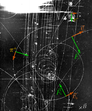
In physics, specifically in electromagnetism, the Lorentz force is the combination of electric and magnetic force on a point charge due to electromagnetic fields. A particle of charge q moving with a velocity v in an electric field E and a magnetic field B experiences a force of

In particle physics, the Dirac equation is a relativistic wave equation derived by British physicist Paul Dirac in 1928. In its free form, or including electromagnetic interactions, it describes all spin-12 massive particles, called "Dirac particles", such as electrons and quarks for which parity is a symmetry. It is consistent with both the principles of quantum mechanics and the theory of special relativity, and was the first theory to account fully for special relativity in the context of quantum mechanics. It was validated by accounting for the fine structure of the hydrogen spectrum in a completely rigorous way.

<span class="mw-page-title-main">Navier–Stokes equations</span> Equations describing the motion of viscous fluid substances

The Navier–Stokes equations are partial differential equations which describe the motion of viscous fluid substances. They were named after French engineer and physicist Claude-Louis Navier and the Irish physicist and mathematician George Gabriel Stokes. They were developed over several decades of progressively building the theories, from 1822 (Navier) to 1842–1850 (Stokes).

<span class="mw-page-title-main">Potential flow</span> Velocity field as the gradient of a scalar function

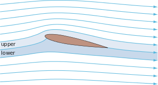
In fluid dynamics, potential flow or irrotational flow refers to a description of a fluid flow with no vorticity in it. Such a description typically arises in the limit of vanishing viscosity, i.e., for an inviscid fluid and with no vorticity present in the flow.

<span class="mw-page-title-main">Stress–energy tensor</span> Tensor describing energy momentum density in spacetime

The stress–energy tensor, sometimes called the stress–energy–momentum tensor or the energy–momentum tensor, is a tensor physical quantity that describes the density and flux of energy and momentum in spacetime, generalizing the stress tensor of Newtonian physics. It is an attribute of matter, radiation, and non-gravitational force fields. This density and flux of energy and momentum are the sources of the gravitational field in the Einstein field equations of general relativity, just as mass density is the source of such a field in Newtonian gravity.

Geometrical optics, or ray optics, is a model of optics that describes light propagation in terms of rays. The ray in geometrical optics is an abstraction useful for approximating the paths along which light propagates under certain circumstances.

<span class="mw-page-title-main">Electromagnetic four-potential</span> Relativistic vector field

An electromagnetic four-potential is a relativistic vector function from which the electromagnetic field can be derived. It combines both an electric scalar potential and a magnetic vector potential into a single four-vector.

In physics, the Hamilton–Jacobi equation, named after William Rowan Hamilton and Carl Gustav Jacob Jacobi, is an alternative formulation of classical mechanics, equivalent to other formulations such as Newton's laws of motion, Lagrangian mechanics and Hamiltonian mechanics.

<span class="mw-page-title-main">Magnetic vector potential</span> Integral of the magnetic field

In classical electromagnetism, magnetic vector potential is the vector quantity defined so that its curl is equal to the magnetic field: . Together with the electric potential φ, the magnetic vector potential can be used to specify the electric field E as well. Therefore, many equations of electromagnetism can be written either in terms of the fields E and B, or equivalently in terms of the potentials φ and A. In more advanced theories such as quantum mechanics, most equations use potentials rather than fields.

In differential geometry, the four-gradient is the four-vector analogue of the gradient from vector calculus.

<span class="mw-page-title-main">Electromagnetic tensor</span> Mathematical object that describes the electromagnetic field in spacetime

In electromagnetism, the electromagnetic tensor or electromagnetic field tensor is a mathematical object that describes the electromagnetic field in spacetime. The field tensor was first used after the four-dimensional tensor formulation of special relativity was introduced by Hermann Minkowski. The tensor allows related physical laws to be written very concisely, and allows for the quantization of the electromagnetic field by Lagrangian formulation described below.

One of the guiding principles in modern chemical dynamics and spectroscopy is that the motion of the nuclei in a molecule is slow compared to that of its electrons. This is justified by the large disparity between the mass of an electron, and the typical mass of a nucleus and leads to the Born–Oppenheimer approximation and the idea that the structure and dynamics of a chemical species are largely determined by nuclear motion on potential energy surfaces.

The electromagnetic wave equation is a second-order partial differential equation that describes the propagation of electromagnetic waves through a medium or in a vacuum. It is a three-dimensional form of the wave equation. The homogeneous form of the equation, written in terms of either the electric field E or the magnetic field B, takes the form:

<span class="mw-page-title-main">Covariant formulation of classical electromagnetism</span> Ways of writing certain laws of physics

The covariant formulation of classical electromagnetism refers to ways of writing the laws of classical electromagnetism in a form that is manifestly invariant under Lorentz transformations, in the formalism of special relativity using rectilinear inertial coordinate systems. These expressions both make it simple to prove that the laws of classical electromagnetism take the same form in any inertial coordinate system, and also provide a way to translate the fields and forces from one frame to another. However, this is not as general as Maxwell's equations in curved spacetime or non-rectilinear coordinate systems.

<span class="mw-page-title-main">Maxwell's equations in curved spacetime</span> Electromagnetism in general relativity

In physics, Maxwell's equations in curved spacetime govern the dynamics of the electromagnetic field in curved spacetime or where one uses an arbitrary coordinate system. These equations can be viewed as a generalization of the vacuum Maxwell's equations which are normally formulated in the local coordinates of flat spacetime. But because general relativity dictates that the presence of electromagnetic fields induce curvature in spacetime, Maxwell's equations in flat spacetime should be viewed as a convenient approximation.

<span class="mw-page-title-main">Inhomogeneous electromagnetic wave equation</span> Equation in physics

In electromagnetism and applications, an inhomogeneous electromagnetic wave equation, or nonhomogeneous electromagnetic wave equation, is one of a set of wave equations describing the propagation of electromagnetic waves generated by nonzero source charges and currents. The source terms in the wave equations make the partial differential equations inhomogeneous, if the source terms are zero the equations reduce to the homogeneous electromagnetic wave equations. The equations follow from Maxwell's equations.

The gradient theorem, also known as the fundamental theorem of calculus for line integrals, says that a line integral through a gradient field can be evaluated by evaluating the original scalar field at the endpoints of the curve. The theorem is a generalization of the second fundamental theorem of calculus to any curve in a plane or space rather than just the real line.

In mathematical physics, spacetime algebra (STA) is the application of Clifford algebra Cl1,3(R), or equivalently the geometric algebra G(M4) to physics. Spacetime algebra provides a "unified, coordinate-free formulation for all of relativistic physics, including the Dirac equation, Maxwell equation and General Relativity" and "reduces the mathematical divide between classical, quantum and relativistic physics."

<span class="mw-page-title-main">Classical electromagnetism and special relativity</span> Relationship between relativity and pre-quantum electromagnetism

The theory of special relativity plays an important role in the modern theory of classical electromagnetism. It gives formulas for how electromagnetic objects, in particular the electric and magnetic fields, are altered under a Lorentz transformation from one inertial frame of reference to another. It sheds light on the relationship between electricity and magnetism, showing that frame of reference determines if an observation follows electric or magnetic laws. It motivates a compact and convenient notation for the laws of electromagnetism, namely the "manifestly covariant" tensor form.

Lagrangian field theory is a formalism in classical field theory. It is the field-theoretic analogue of Lagrangian mechanics. Lagrangian mechanics is used to analyze the motion of a system of discrete particles each with a finite number of degrees of freedom. Lagrangian field theory applies to continua and fields, which have an infinite number of degrees of freedom.

References