| Articles about |
| Electromagnetism |
|---|
 |
This article summarizes equations in the theory of electromagnetism.
| Articles about |
| Electromagnetism |
|---|
| |
This article summarizes equations in the theory of electromagnetism.
Here subscripts e and m are used to differ between electric and magnetic charges. The definitions for monopoles are of theoretical interest, although real magnetic dipoles can be described using pole strengths. There are two possible units for monopole strength, Wb (Weber) and A m (Ampere metre). Dimensional analysis shows that magnetic charges relate by qm(Wb) = μ0qm(Am).
| Quantity (common name/s) | (Common) symbol/s | SI units | Dimension |
|---|---|---|---|
| Electric charge | qe, q, Q | C = As | [I][T] |
| Monopole strength, magnetic charge | qm, g, p | Wb or Am | [L]2[M][T]−2 [I]−1 (Wb) [I][L] (Am) |

Contrary to the strong analogy between (classical) gravitation and electrostatics, there are no "centre of charge" or "centre of electrostatic attraction" analogues.
Electric transport
| Quantity (common name/s) | (Common) symbol/s | Defining equation | SI units | Dimension |
|---|---|---|---|---|
| Linear, surface, volumetric charge density | λe for Linear, σe for surface, ρe for volume. | C m−n, n = 1, 2, 3 | [I][T][L]−n | |
| Capacitance | C | V = voltage, not volume. | F = C V−1 | [I]2[T]4[L]−2[M]−1 |
| Electric current | I | A | [I] | |
| Electric current density | J | A m−2 | [I][L]−2 | |
| Displacement current density | Jd | A m−2 | [I][L]−2 | |
| Convection current density | Jc | A m−2 | [I][L]−2 | |
Electric fields
| Quantity (common name/s) | (Common) symbol/s | Defining equation | SI units | Dimension |
|---|---|---|---|---|
| Electric field, field strength, flux density, potential gradient | E | N C−1 = V m−1 | [M][L][T]−3[I]−1 | |
| Electric flux | ΦE | N m2 C−1 | [M][L]3[T]−3[I]−1 | |
| Absolute permittivity; | ε | F m−1 | [I]2 [T]4 [M]−1 [L]−3 | |
| Electric dipole moment | p | a = charge separation directed from -ve to +ve charge | C m | [I][T][L] |
| Electric Polarization, polarization density | P | C m−2 | [I][T][L]−2 | |
| Electric displacement field, flux density | D | C m−2 | [I][T][L]−2 | |
| Electric displacement flux | ΦD | C | [I][T] | |
| Absolute electric potential, EM scalar potential relative to point Theoretical: | φ ,V | V = J C−1 | [M] [L]2 [T]−3 [I]−1 | |
| Voltage, Electric potential difference | Δφ,ΔV | V = J C−1 | [M] [L]2 [T]−3 [I]−1 | |
Magnetic transport
| Quantity (common name/s) | (Common) symbol/s | Defining equation | SI units | Dimension |
|---|---|---|---|---|
| Linear, surface, volumetric pole density | λm for Linear, σm for surface, ρm for volume. | Wb m−n A m(−n + 1), | [L]2[M][T]−2 [I]−1 (Wb) [I][L] (Am) | |
| Monopole current | Im | Wb s−1 A m s−1 | [L]2[M][T]−3 [I]−1 (Wb) [I][L][T]−1 (Am) | |
| Monopole current density | Jm | Wb s−1 m−2 A m−1 s−1 | [M][T]−3 [I]−1 (Wb) [I][L]−1[T]−1 (Am) | |
Magnetic fields
| Quantity (common name/s) | (Common) symbol/s | Defining equation | SI units | Dimension |
|---|---|---|---|---|
| Magnetic field, field strength, flux density, induction field | B | T = N A−1 m−1 = Wb m−2 | [M][T]−2[I]−1 | |
| Magnetic potential, EM vector potential | A | T m = N A−1 = Wb m3 | [M][L][T]−2[I]−1 | |
| Magnetic flux | ΦB | Wb = T m2 | [L]2[M][T]−2[I]−1 | |
| Magnetic permeability | V·s·A−1·m−1 = N·A−2 = T·m·A−1 = Wb·A−1·m−1 | [M][L][T]−2[I]−2 | ||
| Magnetic moment, magnetic dipole moment | m, μB, Π | Two definitions are possible: using pole strengths, using currents: a = pole separation N is the number of turns of conductor | A m2 | [I][L]2 |
| Magnetization | M | A m−1 | [I] [L]−1 | |
| Magnetic field intensity, (AKA field strength) | H | Two definitions are possible: most common: using pole strengths, [1] | A m−1 | [I] [L]−1 |
| Intensity of magnetization, magnetic polarization | I, J | T = N A−1 m−1 = Wb m−2 | [M][T]−2[I]−1 | |
| Self Inductance | L | Two equivalent definitions are possible: | H = Wb A−1 | [L]2 [M] [T]−2 [I]−2 |
| Mutual inductance | M | Again two equivalent definitions are possible: 1,2 subscripts refer to two conductors/inductors mutually inducing voltage/ linking magnetic flux through each other. They can be interchanged for the required conductor/inductor; | H = Wb A−1 | [L]2 [M] [T]−2 [I]−2 |
| Gyromagnetic ratio (for charged particles in a magnetic field) | γ | Hz T−1 | [M]−1[T][I] | |
DC circuits, general definitions
| Quantity (common name/s) | (Common) symbol/s | Defining equation | SI units | Dimension |
|---|---|---|---|---|
| Terminal Voltage for | Vter | V = J C−1 | [M] [L]2 [T]−3 [I]−1 | |
| Load Voltage for Circuit | Vload | V = J C−1 | [M] [L]2 [T]−3 [I]−1 | |
| Internal resistance of power supply | Rint | Ω = V A−1 = J s C−2 | [M][L]2 [T]−3 [I]−2 | |
| Load resistance of circuit | Rext | Ω = V A−1 = J s C−2 | [M][L]2 [T]−3 [I]−2 | |
| Electromotive force (emf), voltage across entire circuit including power supply, external components and conductors | E | V = J C−1 | [M] [L]2 [T]−3 [I]−1 | |
AC circuits
| Quantity (common name/s) | (Common) symbol/s | Defining equation | SI units | Dimension |
|---|---|---|---|---|
| Resistive load voltage | VR | V = J C−1 | [M] [L]2 [T]−3 [I]−1 | |
| Capacitive load voltage | VC | V = J C−1 | [M] [L]2 [T]−3 [I]−1 | |
| Inductive load voltage | VL | V = J C−1 | [M] [L]2 [T]−3 [I]−1 | |
| Capacitive reactance | XC | Ω−1 m−1 | [I]2 [T]3 [M]−2 [L]−2 | |
| Inductive reactance | XL | Ω−1 m−1 | [I]2 [T]3 [M]−2 [L]−2 | |
| AC electrical impedance | Z | Ω−1 m−1 | [I]2 [T]3 [M]−2 [L]−2 | |
| Phase constant | δ, φ | dimensionless | dimensionless | |
| AC peak current | I0 | A | [I] | |
| AC root mean square current | Irms | A | [I] | |
| AC peak voltage | V0 | V = J C−1 | [M] [L]2 [T]−3 [I]−1 | |
| AC root mean square voltage | Vrms | V = J C−1 | [M] [L]2 [T]−3 [I]−1 | |
| AC emf, root mean square | V = J C−1 | [M] [L]2 [T]−3 [I]−1 | ||
| AC average power | W = J s−1 | [M] [L]2 [T]−3 | ||
| Capacitive time constant | τC | s | [T] | |
| Inductive time constant | τL | s | [T] | |
| Quantity (common name/s) | (Common) symbol/s | Defining equation | SI units | Dimension |
|---|---|---|---|---|
| Magnetomotive force, mmf | F, | N = number of turns of conductor | A | [I] |
General Classical Equations
| Physical situation | Equations |
|---|---|
| Electric potential gradient and field | |
| Point charge | |
| At a point in a local array of point charges | |
| At a point due to a continuum of charge | |
| Electrostatic torque and potential energy due to non-uniform fields and dipole moments | |
General classical equations
| Physical situation | Equations |
|---|---|
| Magnetic potential, EM vector potential | |
| Due to a magnetic moment | |
| Magnetic moment due to a current distribution | |
| Magnetostatic torque and potential energy due to non-uniform fields and dipole moments | |
Below N = number of conductors or circuit components. Subscript net refers to the equivalent and resultant property value.
| Physical situation | Nomenclature | Series | Parallel |
|---|---|---|---|
| Resistors and conductors |
| ||
| Charge, capacitors, currents |
| ||
| Inductors |
| ||
| Circuit | DC Circuit equations | AC Circuit equations |
|---|---|---|
| RC circuits | Circuit equation Capacitor charge Capacitor discharge | |
| RL circuits | Circuit equation Inductor current rise Inductor current fall | |
| LC circuits | Circuit equation | Circuit equation Circuit resonant frequency Circuit charge Circuit current Circuit electrical potential energy Circuit magnetic potential energy |
| RLC Circuits | Circuit equation | Circuit equation Circuit charge |

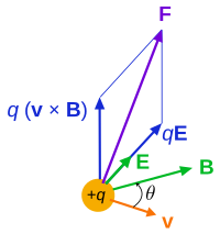
In physics, electromagnetism is an interaction that occurs between particles with electric charge via electromagnetic fields. The electromagnetic force is one of the four fundamental forces of nature. It is the dominant force in the interactions of atoms and molecules. Electromagnetism can be thought of as a combination of electrostatics and magnetism, which are distinct but closely intertwined phenomena. Electromagnetic forces occur between any two charged particles. Electric forces cause an attraction between particles with opposite charges and repulsion between particles with the same charge, while magnetism is an interaction that occurs between charged particles in relative motion. These two forces are described in terms of electromagnetic fields. Macroscopic charged objects are described in terms of Coulomb's law for electricity and Ampère's force law for magnetism; the Lorentz force describes microscopic charged particles.

An electromagnetic field is a physical field, mathematical functions of position and time, representing the influences on and due to electric charges. The field at any point in space and time can be regarded as a combination of an electric field and a magnetic field. Because of the interrelationship between the fields, a disturbance in the electric field can create a disturbance in the magnetic field which in turn affects the electric field, leading to an oscillation that propagates through space, known as an electromagnetic wave.

Mathematical physics refers to the development of mathematical methods for application to problems in physics. The Journal of Mathematical Physics defines the field as "the application of mathematics to problems in physics and the development of mathematical methods suitable for such applications and for the formulation of physical theories". An alternative definition would also include those mathematics that are inspired by physics, known as physical mathematics.

In particle physics, a magnetic monopole is a hypothetical elementary particle that is an isolated magnet with only one magnetic pole. A magnetic monopole would have a net north or south "magnetic charge". Modern interest in the concept stems from particle theories, notably the grand unified and superstring theories, which predict their existence. The known elementary particles that have electric charge are electric monopoles.
In physics, chemistry and biology, a potential gradient is the local rate of change of the potential with respect to displacement, i.e. spatial derivative, or gradient. This quantity frequently occurs in equations of physical processes because it leads to some form of flux.
In physics, semiclassical refers to a theory in which one part of a system is described quantum mechanically, whereas the other is treated classically. For example, external fields will be constant, or when changing will be classically described. In general, it incorporates a development in powers of Planck's constant, resulting in the classical physics of power 0, and the first nontrivial approximation to the power of (−1). In this case, there is a clear link between the quantum-mechanical system and the associated semi-classical and classical approximations, as it is similar in appearance to the transition from physical optics to geometric optics.
In theoretical physics and applied mathematics, a field equation is a partial differential equation which determines the dynamics of a physical field, specifically the time evolution and spatial distribution of the field. The solutions to the equation are mathematical functions which correspond directly to the field, as functions of time and space. Since the field equation is a partial differential equation, there are families of solutions which represent a variety of physical possibilities. Usually, there is not just a single equation, but a set of coupled equations which must be solved simultaneously. Field equations are not ordinary differential equations since a field depends on space and time, which requires at least two variables.
Magnetic scalar potential, ψ, is a quantity in classical electromagnetism analogous to electric potential. It is used to specify the magnetic H-field in cases when there are no free currents, in a manner analogous to using the electric potential to determine the electric field in electrostatics. One important use of ψ is to determine the magnetic field due to permanent magnets when their magnetization is known. The potential is valid in any region with zero current density, thus if currents are confined to wires or surfaces, piecemeal solutions can be stitched together to provide a description of the magnetic field at all points in space.
In physics, Gauss's law for magnetism is one of the four Maxwell's equations that underlie classical electrodynamics. It states that the magnetic field B has divergence equal to zero, in other words, that it is a solenoidal vector field. It is equivalent to the statement that magnetic monopoles do not exist. Rather than "magnetic charges", the basic entity for magnetism is the magnetic dipole.
In physics, relativistic quantum mechanics (RQM) is any Poincaré covariant formulation of quantum mechanics (QM). This theory is applicable to massive particles propagating at all velocities up to those comparable to the speed of light c, and can accommodate massless particles. The theory has application in high energy physics, particle physics and accelerator physics, as well as atomic physics, chemistry and condensed matter physics. Non-relativistic quantum mechanics refers to the mathematical formulation of quantum mechanics applied in the context of Galilean relativity, more specifically quantizing the equations of classical mechanics by replacing dynamical variables by operators. Relativistic quantum mechanics (RQM) is quantum mechanics applied with special relativity. Although the earlier formulations, like the Schrödinger picture and Heisenberg picture were originally formulated in a non-relativistic background, a few of them also work with special relativity.

In physics, a field is a physical quantity, represented by a scalar, vector, or tensor, that has a value for each point in space and time. For example, on a weather map, the surface temperature is described by assigning a number to each point on the map; the temperature can be considered at a certain point in time or over some interval of time, to study the dynamics of temperature change. A surface wind map, assigning an arrow to each point on a map that describes the wind speed and direction at that point, is an example of a vector field, i.e. a 1-dimensional (rank-1) tensor field. Field theories, mathematical descriptions of how field values change in space and time, are ubiquitous in physics. For instance, the electric field is another rank-1 tensor field, while electrodynamics can be formulated in terms of two interacting vector fields at each point in spacetime, or as a single-rank 2-tensor field.

Classical Electrodynamics is a textbook written by theoretical particle and nuclear physicist John David Jackson. The book originated as lecture notes that Jackson prepared for teaching graduate-level electromagnetism first at McGill University and then at the University of Illinois at Urbana-Champaign. Intended for graduate students, and often known as Jackson for short, it has been a standard reference on its subject since its first publication in 1962.
Electromagnetism is one of the fundamental forces of nature. Early on, electricity and magnetism were studied separately and regarded as separate phenomena. Hans Christian Ørsted discovered that the two were related – electric currents give rise to magnetism. Michael Faraday discovered the converse, that magnetism could induce electric currents, and James Clerk Maxwell put the whole thing together in a unified theory of electromagnetism. Maxwell's equations further indicated that electromagnetic waves existed, and the experiments of Heinrich Hertz confirmed this, making radio possible. Maxwell also postulated, correctly, that light was a form of electromagnetic wave, thus making all of optics a branch of electromagnetism. Radio waves differ from light only in that the wavelength of the former is much longer than the latter. Albert Einstein showed that the magnetic field arises through the relativistic motion of the electric field and thus magnetism is merely a side effect of electricity. The modern theoretical treatment of electromagnetism is as a quantum field in quantum electrodynamics.


