Persistent data structure

Not to be confused with Persistent storage.

In computing, a persistent data structure or not ephemeral data structure is a data structure that always preserves the previous version of itself when it is modified. Such data structures are effectively immutable, as their operations do not (visibly) update the structure in-place, but instead always yield a new updated structure. The term was introduced in Driscoll, Sarnak, Sleator, and Tarjan's 1986 article. ^[1]

A data structure is partially persistent if all versions can be accessed but only the newest version can be modified. The data structure is fully persistent if every version can be both accessed and modified. If there is also a meld or merge operation that can create a new version from two previous versions, the data structure is called confluently persistent. Structures that are not persistent are called ephemeral. ^[2]

These types of data structures are particularly common in logical and functional programming, ^[2] as languages in those paradigms discourage (or fully forbid) the use of mutable data.

Partial versus full persistence

In the partial persistence model, a programmer may query any previous version of a data structure, but may only update the latest version. This implies a linear ordering among each version of the data structure. ^[3] In the fully persistent model, both updates and queries are allowed on any version of the data structure. In some cases the performance characteristics of querying or updating older versions of a data structure may be allowed to degrade, as is true with the rope data structure. ^[4] In addition, a data structure can be referred to as confluently persistent if, in addition to being fully persistent, two versions of the same data structure can be combined to form a new version which is still fully persistent. ^[5]

Partially persistent data structure

A type of data structure where user may query any version of the structure but may only update the latest version.

An ephermeral data structure can be converted to partially persistent data structure using a few techniques.

One of the technique is by using randomized version of Van Emde Boas Tree which is created using dynamic perfect hashing. This data structure is created as follows:

• A stratified tree with m elements is implemented using dynamic perfect hashing.
• The tree is pruned by dividing the m elements into buckets of size log(log n) such that the elements of bucket 1 is smaller than the elements of bucket 2 and so on.
• The maximal element in each bucket is stored in the stratified tree and each bucket is stored in the structure as an unordered linked list.

The size of this data structure is bounded by the number of elements stored in the structure that is O(m). The insertion of a new maximal element is done in constant O(1) expected and amortized time. Finally query to find an element can be done in this structure in O(log(log n)) worst-case time. ^[6]

Techniques for preserving previous versions

Copy-on-write

One method for creating a persistent data structure is to use a platform provided ephemeral data structure such as an array to store the data in the data structure and copy the entirety of that data structure using copy-on-write semantics for any updates to the data structure. This is an inefficient technique because the entire backing data structure must be copied for each write, leading to worst case O(n·m) performance characteristics for m modifications of an array of size n.^{[ citation needed ]}

Fat node

The fat node method is to record all changes made to node fields in the nodes themselves, without erasing old values of the fields. This requires that nodes be allowed to become arbitrarily “fat”. In other words, each fat node contains the same information and pointer fields as an ephemeral node, along with space for an arbitrary number of extra field values. Each extra field value has an associated field name and a version stamp which indicates the version in which the named field was changed to have the specified value. Besides, each fat node has its own version stamp, indicating the version in which the node was created. The only purpose of nodes having version stamps is to make sure that each node only contains one value per field name per version. In order to navigate through the structure, each original field value in a node has a version stamp of zero.

Complexity of fat node

With using fat node method, it requires O(1) space for every modification: just store the new data. Each modification takes O(1) additional time to store the modification at the end of the modification history. This is an amortized time bound, assuming modification history is stored in a growable array. At access time, the right version at each node must be found as the structure is traversed. If "m" modifications were to be made, then each access operation would have O(log m) slowdown resulting from the cost of finding the nearest modification in the array.

Path copying

With the path copying method a copy of all nodes is made on the path to any node which is about to be modified. These changes must then be cascaded back through the data structure: all nodes that pointed to the old node must be modified to point to the new node instead. These modifications cause more cascading changes, and so on, until the root node is reached.

Complexity of path copying

With m modifications, this costs O(log m) additive lookup time. Modification time and space are bounded by the size of the longest path in the data structure and the cost of the update in the ephemeral data structure. In a Balanced Binary Search Tree without parent pointers the worst case modification time complexity is O(log n + update cost). However, in a linked list the worst case modification time complexity is O(n + update cost).

A combination

Driscoll, Sarnak, Sleator, Tarjan came up ^[1] with a way to combine the techniques of fat nodes and path copying, achieving O(1) access slowdown and O(1) modification space and time complexity.

In each node, one modification box is stored. This box can hold one modification to the node—either a modification to one of the pointers, or to the node's key, or to some other piece of node-specific data—and a timestamp for when that modification was applied. Initially, every node's modification box is empty.

Whenever a node is accessed, the modification box is checked, and its timestamp is compared against the access time. (The access time specifies the version of the data structure being considered.) If the modification box is empty, or the access time is before the modification time, then the modification box is ignored and only the normal part of the node is considered. On the other hand, if the access time is after the modification time, then the value in the modification box is used, overriding that value in the node.

Modifying a node works like this. (It is assumed that each modification touches one pointer or similar field.) If the node's modification box is empty, then it is filled with the modification. Otherwise, the modification box is full. A copy of the node is made, but using only the latest values. The modification is performed directly on the new node, without using the modification box. (One of the new node's fields is overwritten and its modification box stays empty.) Finally, this change is cascaded to the node's parent, just like path copying. (This may involve filling the parent's modification box, or making a copy of the parent recursively. If the node has no parent—it's the root—it is added the new root to a sorted array of roots.)

With this algorithm, given any time t, at most one modification box exists in the data structure with time t. Thus, a modification at time t splits the tree into three parts: one part contains the data from before time t, one part contains the data from after time t, and one part was unaffected by the modification.

Complexity of the combination

Time and space for modifications require amortized analysis. A modification takes O(1) amortized space, and O(1) amortized time. To see why, use a potential function ϕ, where ϕ(T) is the number of full live nodes in T . The live nodes of T are just the nodes that are reachable from the current root at the current time (that is, after the last modification). The full live nodes are the live nodes whose modification boxes are full.

Each modification involves some number of copies, say k, followed by 1 change to a modification box. Consider each of the k copies. Each costs O(1) space and time, but decreases the potential function by one. (First, the node to be copied must be full and live, so it contributes to the potential function. The potential function will only drop, however, if the old node isn't reachable in the new tree. But it is known that it isn't reachable in the new tree—the next step in the algorithm will be to modify the node's parent to point at the copy. Finally, it is known that the copy's modification box is empty. Thus, replaced a full live node has been replaced with an empty live node, and ϕ goes down by one.) The final step fills a modification box, which costs O(1) time and increases ϕ by one.

Putting it all together, the change in ϕ is Δϕ =1− k. Thus, the algorithm takes O(k +Δϕ)= O(1) space and O(k +Δϕ +1) = O(1) time

Generalized form of persistence

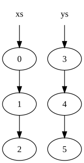
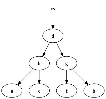
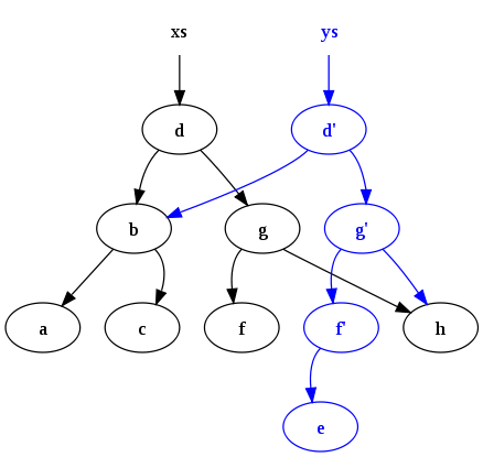
Path copying is one of the simple methods to achieve persistency in a certain data structure such as binary search trees. It is nice to have a general strategy for implementing persistence that works with any given data structure. In order to achieve that, we consider a directed graph G. We assume that each vertex v in G has a constant number c of outgoing edges that are represented by pointers. Each vertex has a label representing the data. We consider that a vertex has a bounded number d of edges leading into it which we define as inedges(v). We allow the following different operations on G.

• CREATE-NODE(): Creates a new vertex with no incoming or outgoing edges.
• CHANGE-EDGE(v, i, u): Changes the i^th edge of v to point to u
• CHANGE-LABEL(v, x): Changes the value of the data stored at v to x

Any of the above operations is performed at a specific time and the purpose of the persistent graph representation is to be able to access any version of G at any given time. For this purpose we define a table for each vertex v in G. The table contains c columns and ${\displaystyle d+1}$ rows. Each row contains in addition to the pointers for the outgoing edges, a label which represents the data at the vertex and a time t at which the operation was performed. In addition to that there is an array inedges(v) that keeps track of all the incoming edges to v. When a table is full, a new table with ${\displaystyle d+1}$ rows can be created. The old table becomes inactive and the new table becomes the active table.

CREATE-NODE

A call to CREATE-NODE creates a new table and set all the references to null

CHANGE-EDGE

If we assume that CHANGE-EDGE(v, i, u) is called, then there are two cases to consider.

• There is an empty row in the table of the vertex v: In this case we copy the last row in the table and we change the ith edge of vertex v to point to the new vertex u
• Table of the vertex v is full: In this case we need to create a new table. We copy the last row of the old table into the new table. We need to loop in the array inedges(v) in order to let each vertex in the array point to the new table created. In addition to that, we need to change the entry v in the inedges(w) for every vertex w such that edge v,w exists in the graph G.

CHANGE-LABEL

It works exactly the same as CHANGE-EDGE except that instead of changing the i^th edge of the vertex, we change the i^th label.

Efficiency of the generalized persistent data structure

In order to find the efficiency of the scheme proposed above, we use an argument defined as a credit scheme. The credit represents a currency. For example, the credit can be used to pay for a table. The argument states the following:

• The creation of one table requires one credit
• Each call to CREATE-NODE comes with two credits
• Each call to CHANGE-EDGE comes with one credit

The credit scheme should always satisfy the following invariant: Each row of each active table stores one credit and the table has the same number of credits as the number of rows. Let us confirm that the invariant applies to all the three operations CREATE-NODE, CHANGE-EDGE and CHANGE-LABEL.

• CREATE-NODE: It acquires two credits, one is used to create the table and the other is given to the one row that is added to the table. Thus the invariant is maintained.
• CHANGE-EDGE: There are two cases to consider. The first case occurs when there is still at least one empty row in the table. In this case one credit is used to the newly inserted row. The second case occurs when the table is full. In this case the old table becomes inactive and the ${\displaystyle d+1}$ credits are transformed to the new table in addition to the one credit acquired from calling the CHANGE-EDGE. So in total we have ${\displaystyle d+2}$ credits. One credit will be used for the creation of the new table. Another credit will be used for the new row added to the table and the d credits left are used for updating the tables of the other vertices that need to point to the new table. We conclude that the invariant is maintained.
• CHANGE-LABEL: It works exactly the same as CHANGE-EDGE.

As a summary, we conclude that having ${\displaystyle n_{1}}$ calls to CREATE_NODE and ${\displaystyle n_{2}}$ calls to CHANGE_EDGE will result in the creation of ${\displaystyle 2\cdot n_{1}+n_{2}}$ tables. Since each table has size ${\displaystyle O(d)}$ without taking into account the recursive calls, then filling in a table requires ${\displaystyle O(d^{2})}$ where the additional d factor comes from updating the inedges at other nodes. Therefore, the amount of work required to complete a sequence of operations is bounded by the number of tables created multiplied by ${\displaystyle O(d^{2})}$. Each access operation can be done in ${\displaystyle O(Log(d))}$ and there are ${\displaystyle m}$ edge and label operations, thus it requires ${\displaystyle m\cdot O(Log(d))}$. We conclude that There exists a data structure that can complete any ${\displaystyle n}$ sequence of CREATE-NODE, CHANGE-EDGE and CHANGE-LABEL in ${\displaystyle O(n\cdot d^{2})+m\cdot O(Log(d))}$.

Applications of persistent data structures

Next element search or point location

One of the useful applications that can be solved efficiently using persistence is the Next Element Search. Assume that there are ${\displaystyle n}$ non intersecting line segments that don't cross each other that are parallel to the x-axis. We want to build a data structure that can query a point ${\displaystyle p}$ and return the segment above ${\displaystyle p}$ (if any). We will start by solving the Next Element Search using the naïve method then we will show how to solve it using the persistent data structure method.

Naïve method

We start with a vertical line segment that starts off at infinity and we sweep the line segments from the left to the right. We take a pause every time we encounter an end point of these segments. The vertical lines split the plane into vertical strips. If there are ${\displaystyle n}$ line segments then we can get ${\displaystyle 2\cdot n+1}$ vertical strips since each segment has ${\displaystyle 2}$ end points. No segment begins and ends in the strip. Every segment either it doesn't touch the strip or it completely crosses it. We can think of the segments as some objects that are in some sorted order from top to bottom. What we care about is where the point that we are looking at fits in this order. We sort the endpoints of the segments by their ${\displaystyle x}$ coordinate. For each strip ${\displaystyle s_{i}}$, we store the subset segments that cross ${\displaystyle s_{i}}$ in a dictionary. When the vertical line sweeps the line segments, whenever it passes over the left endpoint of a segment then we add it to the dictionary. When it passes through the right endpoint of the segment, we remove it from the dictionary. At every endpoint, we save a copy of the dictionary and we store all the copies sorted by the ${\displaystyle x}$ coordinates. Thus we have a data structure that can answer any query. In order to find the segment above a point ${\displaystyle p}$, we can look at the ${\displaystyle x}$ coordinate of ${\displaystyle p}$ to know which copy or strip it belongs to. Then we can look at the ${\displaystyle y}$ coordinate to find the segment above it. Thus we need two binary searches, one for the ${\displaystyle x}$ coordinate to find the strip or the copy, and another for the ${\displaystyle y}$ coordinate to find the segment above it. Thus the query time takes ${\displaystyle O(Log(n))}$. In this data structure, the space is the issue since if we assume that we have the segments structured in a way such that every segment starts before the end of any other segment, then the space required for the structure to be built using the naïve method would be ${\displaystyle O(n^{2})}$. Let us see how we can build another persistent data structure with the same query time but with a better space.

Persistent data structure method

We can notice that what really takes time in the data structure used in the naïve method is that whenever we move from a strip to the next, we need to take a snap shot of whatever data structure we are using to keep things in sorted order. We can notice that once we get the segments that intersect ${\displaystyle s_{i}}$, when we move to ${\displaystyle s_{i+1}}$ either one thing leaves or one thing enters. If the difference between what is in ${\displaystyle s_{i}}$ and what is in ${\displaystyle s_{i+1}}$ is only one insertion or deletion then it is not a good idea to copy everything from ${\displaystyle s_{i}}$ to ${\displaystyle s_{i+1}}$. The trick is that since each copy differs from the previous one by only one insertion or deletion, then we need to copy only the parts that change. Let us assume that we have a tree rooted at ${\displaystyle T}$. When we insert a key ${\displaystyle k}$ into the tree, we create a new leaf containing ${\displaystyle k}$. Performing rotations to rebalance the tree will only modify the nodes of the path from ${\displaystyle k}$ to ${\displaystyle T}$. Before inserting the key ${\displaystyle k}$ into the tree, we copy all the nodes on the path from ${\displaystyle k}$ to ${\displaystyle T}$. Now we have 2 versions of the tree, the original one which doesn't contain ${\displaystyle k}$ and the new tree that contains ${\displaystyle k}$ and whose root is a copy of the root of ${\displaystyle T}$. Since copying the path from ${\displaystyle k}$ to ${\displaystyle T}$ doesn't increase the insertion time by more than a constant factor then the insertion in the persistent data structure takes ${\displaystyle O(Log(n))}$ time. For the deletion, we need to find which nodes will be affected by the deletion. For each node ${\displaystyle v}$ affected by the deletion, we copy the path from the root to ${\displaystyle v}$. This will provide a new tree whose root is a copy of the root of the original tree. Then we perform the deletion on the new tree. We will end up with 2 versions of the tree. The original one which contains ${\displaystyle k}$ and the new one which doesn't contain ${\displaystyle k}$. Since any deletion only modifies the path from the root to ${\displaystyle v}$ and any appropriate deletion algorithm runs in ${\displaystyle O(Log(n))}$, thus the deletion in the persistent data structure takes ${\displaystyle O(Log(n))}$. Every sequence of insertion and deletion will cause the creation of a sequence of dictionaries or versions or trees ${\displaystyle S_{1},S_{2},\dots S_{i}}$ where each ${\displaystyle S_{i}}$ is the result of operations ${\displaystyle S_{1},S_{2},\dots S_{i}}$. If each ${\displaystyle S_{i}}$ contains ${\displaystyle m}$ elements, then the search in each ${\displaystyle S_{i}}$ takes ${\displaystyle O(Log(m))}$. Using this persistent data structure we can solve the next element search problem in ${\displaystyle O(Log(n))}$ query time and ${\displaystyle O(n\cdot Log(n))}$ space instead of ${\displaystyle O(n^{2})}$. Please find below the source code for an example related to the next search problem.

Examples of persistent data structures

Perhaps the simplest persistent data structure is the singly linked list or cons-based list, a simple list of objects formed by each carrying a reference to the next in the list. This is persistent because the tail of the list can be taken, meaning the last k items for some k, and new nodes can be added in front of it. The tail will not be duplicated, instead becoming shared between both the old list and the new list. So long as the contents of the tail are immutable, this sharing will be invisible to the program.

Many common reference-based data structures, such as red–black trees, ^[7] stacks, ^[8] and treaps, ^[9] can easily be adapted to create a persistent version. Some others need slightly more effort, for example: queues, dequeues, and extensions including min-deques (which have an additional O(1) operation min returning the minimal element) and random access deques (which have an additional operation of random access with sub-linear, most often logarithmic, complexity).

There also exist persistent data structures which use destructive^{[ clarification needed ]} operations, making them impossible to implement efficiently in purely functional languages (like Haskell outside specialized monads like state or IO), but possible in languages like C or Java. These types of data structures can often be avoided with a different design. One primary advantage to using purely persistent data structures is that they often behave better in multi-threaded environments.

Linked lists

Singly linked lists are the bread-and-butter data structure in functional languages. ^[10] Some ML-derived languages, like Haskell, are purely functional because once a node in the list has been allocated, it cannot be modified, only copied, referenced or destroyed by the garbage collector when nothing refers to it. (Note that ML itself is not purely functional, but supports non-destructive list operations subset, that is also true in the Lisp (LISt Processing) functional language dialects like Scheme and Racket.)

Consider the two lists:

xs = [0, 1, 2] ys = [3, 4, 5]

These would be represented in memory by:

where a circle indicates a node in the list (the arrow out representing the second element of the node which is a pointer to another node).

Now concatenating the two lists:

zs = xs ++ ys

results in the following memory structure:

Notice that the nodes in list xs have been copied, but the nodes in ys are shared. As a result, the original lists (xs and ys) persist and have not been modified.

The reason for the copy is that the last node in xs (the node containing the original value 2) cannot be modified to point to the start of ys, because that would change the value of xs.

Trees

Consider a binary search tree, ^[10] where every node in the tree has the recursive invariant that all subnodes contained in the left subtree have a value that is less than or equal to the value stored in the node, and subnodes contained in the right subtree have a value that is greater than the value stored in the node.

For instance, the set of data

xs = [a, b, c, d, f, g, h]

might be represented by the following binary search tree:

A function which inserts data into the binary tree and maintains the invariant is:

funinsert(x,E)=T(E,x,E)|insert(x,sasT(a,y,b))=ifx<ythenT(insert(x,a),y,b)elseifx>ythenT(a,y,insert(x,b))elses

After executing

ys = insert ("e", xs)

The following configuration is produced:

Notice two points: first, the original tree (xs) persists. Second, many common nodes are shared between the old tree and the new tree. Such persistence and sharing is difficult to manage without some form of garbage collection (GC) to automatically free up nodes which have no live references, and this is why GC is a feature commonly found in functional programming languages.

Code

Github repo containing implementations of persistent BSTs using Fat Nodes, Copy-on-Write, and Path Copying Techniques.

To use the persistent BST implementations, simply clone the repository and follow the instructions provided in the README file.

Link: https://github.com/DesaultierMAKK/PersistentBST

Persistent hash array mapped trie

A persistent hash array mapped trie is a specialized variant of a hash array mapped trie that will preserve previous versions of itself on any updates. It is often used to implement a general purpose persistent map data structure. ^[11]

Hash array mapped tries were originally described in a 2001 paper by Phil Bagwell entitled "Ideal Hash Trees". This paper presented a mutable Hash table where "Insert, search and delete times are small and constant, independent of key set size, operations are O(1). Small worst-case times for insert, search and removal operations can be guaranteed and misses cost less than successful searches". ^[12] This data structure was then modified by Rich Hickey to be fully persistent for use in the Clojure programming language. ^[13]

Conceptually, hash array mapped tries work similar to any generic tree in that they store nodes hierarchically and retrieve them by following a path down to a particular element. The key difference is that Hash Array Mapped Tries first use a hash function to transform their lookup key into a (usually 32 or 64 bit) integer. The path down the tree is then determined by using slices of the binary representation of that integer to index into a sparse array at each level of the tree. The leaf nodes of the tree behave similar to the buckets used to construct hash tables and may or may not contain multiple candidates depending on hash collisions. ^[11]

Most implementations of persistent hash array mapped tries use a branching factor of 32 in their implementation. This means that in practice while insertions, deletions, and lookups into a persistent hash array mapped trie have a computational complexity of O(log n), for most applications they are effectively constant time, as it would require an extremely large number of entries to make any operation take more than a dozen steps. ^[14]

Usage in programming languages

Haskell

Haskell is a pure functional language and therefore does not allow for mutation. Therefore, all data structures in the language are persistent, as it is impossible to not preserve the previous state of a data structure with functional semantics. ^[15] This is because any change to a data structure that would render previous versions of a data structure invalid would violate referential transparency.

In its standard library Haskell has efficient persistent implementations for linked lists, ^[16] Maps (implemented as size balanced trees), ^[17] and Sets ^[18] among others. ^[19]

Clojure

Like many programming languages in the Lisp family, Clojure contains an implementation of a linked list, but unlike other dialects its implementation of a linked list has enforced persistence instead of being persistent by convention. ^[20] Clojure also has efficient implementations of persistent vectors, maps, and sets based on persistent hash array mapped tries. These data structures implement the mandatory read-only parts of the Java collections framework. ^[21]

The designers of the Clojure language advocate the use of persistent data structures over mutable data structures because they have value semantics which gives the benefit of making them freely shareable between threads with cheap aliases, easy to fabricate, and language independent. ^[22]

These data structures form the basis of Clojure's support for parallel computing since they allow for easy retries of operations to sidestep data races and atomic compare and swap semantics. ^[23]

Elm

The Elm programming language is purely functional like Haskell, which makes all of its data structures persistent by necessity. It contains persistent implementations of linked lists as well as persistent arrays, dictionaries, and sets. ^[24]

Elm uses a custom virtual DOM implementation that takes advantage of the persistent nature of Elm data. As of 2016 it was reported by the developers of Elm that this virtual DOM allows the Elm language to render HTML faster than the popular JavaScript frameworks React, Ember, and Angular. ^[25]

Java

The Java programming language is not particularly functional. Despite this, the core JDK package java.util.concurrent includes CopyOnWriteArrayList and CopyOnWriteArraySet which are persistent structures, implemented using copy-on-write techniques. The usual concurrent map implementation in Java, ConcurrentHashMap, is not persistent, however. Fully persistent collections are available in third-party libraries, ^[26] or other JVM languages.

JavaScript

The popular JavaScript frontend framework React is frequently used along with a state management system that implements the Flux architecture, ^{[27] [28]} a popular implementation of which is the JavaScript library Redux. The Redux library is inspired by the state management pattern used in the Elm programming language, meaning that it mandates that users treat all data as persistent. ^[29] As a result, the Redux project recommends that in certain cases users make use of libraries for enforced and efficient persistent data structures. This reportedly allows for greater performance than when comparing or making copies of regular JavaScript objects. ^[30]

One such library of persistent data structures Immutable.js is based on the data structures made available and popularized by Clojure and Scala. ^[31] It is mentioned by the documentation of Redux as being one of the possible libraries that can provide enforced immutability. ^[30] Mori.js brings data structures similar to those in Clojure to JavaScript. ^[32] Immer.js brings an interesting approach where one "creates the next immutable state by mutating the current one". ^[33] Immer.js uses native JavaScript objects and not efficient persistent data structures and it might cause performance issues when data size is big.

Prolog

Prolog terms are naturally immutable and therefore data structures are typically persistent data structures. Their performance depends on sharing and garbage collection offered by the Prolog system. ^[34] Extensions to non-ground Prolog terms are not always feasible because of search space explosion. Delayed goals might mitigate the problem.

Some Prolog systems nevertheless do provide destructive operations like setarg/3, which might come in different flavors, with/without copying and with/without backtracking of the state change. There are cases where setarg/3 is used to the good of providing a new declarative layer, like a constraint solver. ^[35]

Scala

The Scala programming language promotes the use of persistent data structures for implementing programs using "Object-Functional Style". ^[36] Scala contains implementations of many persistent data structures including linked lists, red–black trees, as well as persistent hash array mapped tries as introduced in Clojure. ^[37]

Garbage collection

Because persistent data structures are often implemented in such a way that successive versions of a data structure share underlying memory ^[38] ergonomic use of such data structures generally requires some form of automatic garbage collection system such as reference counting or mark and sweep. ^[39] In some platforms where persistent data structures are used it is an option to not use garbage collection which, while doing so can lead to memory leaks, can in some cases have a positive impact on the overall performance of an application. ^[40]

See also

• Copy-on-write
• Navigational database
• Persistent data
• Retroactive data structures
• Purely functional data structure

References

1. Driscoll JR, Sarnak N, Sleator DD, Tarjan RE (1986). "Making data structures persistent". Proceedings of the eighteenth annual ACM symposium on Theory of computing - STOC '86. pp. 109–121. CiteSeerX   10.1.1.133.4630 . doi:10.1145/12130.12142. ISBN   978-0-89791-193-1. S2CID   364871.
2. Kaplan, Haim (2001). "Persistent data structures". Handbook on Data Structures and Applications.
3. Conchon, Sylvain; Filliâtre, Jean-Christophe (2008), "Semi-persistent Data Structures", Programming Languages and Systems, Lecture Notes in Computer Science, vol. 4960, Springer Berlin Heidelberg, pp. 322–336, doi: 10.1007/978-3-540-78739-6_25 , ISBN   9783540787389
4. Tiark, Bagwell, Philip Rompf (2011). RRB-Trees: Efficient Immutable Vectors. OCLC   820379112.
5. Brodal, Gerth Stølting; Makris, Christos; Tsichlas, Kostas (2006), "Purely Functional Worst Case Constant Time Catenable Sorted Lists", Algorithms – ESA 2006, Lecture Notes in Computer Science, vol. 4168, Springer Berlin Heidelberg, pp. 172–183, CiteSeerX   10.1.1.70.1493 , doi:10.1007/11841036_18, ISBN   9783540388753
6. Lenhof, Hans-Peter; Smid, Michiel (1994). "Using persistent data structures for adding range restrictions to searching problems". RAIRO - Theoretical Informatics and Applications. 28 (1): 25–49. doi:10.1051/ita/1994280100251. ISSN   0988-3754.
7. Neil Sarnak; Robert E. Tarjan (1986). "Planar Point Location Using Persistent Search Trees" (PDF). Communications of the ACM. 29 (7): 669–679. doi:10.1145/6138.6151. S2CID   8745316. Archived from the original (PDF) on 2015-10-10. Retrieved 2011-04-06.
8. Chris Okasaki. "Purely Functional Data Structures (thesis)" (PDF).{{cite journal}}: Cite journal requires |journal= (help)
9. Liljenzin, Olle (2013). "Confluently Persistent Sets and Maps". arXiv: 1301.3388 . Bibcode:2013arXiv1301.3388L.{{cite journal}}: Cite journal requires |journal= (help)
10. This example is taken from Okasaki. See the bibliography.
11. BoostCon (2017-06-13), C++Now 2017: Phil Nash "The Holy Grail!? A Persistent Hash-Array-Mapped Trie for C++", archived from the original on 2021-12-21, retrieved 2018-10-22
12. Phil, Bagwell (2001). "Ideal Hash Trees".{{cite journal}}: Cite journal requires |journal= (help)
13. "Are We There Yet?". InfoQ. Retrieved 2018-10-22.
14. Steindorfer, Michael J.; Vinju, Jurgen J. (2015-10-23). "Optimizing hash-array mapped tries for fast and lean immutable JVM collections". ACM SIGPLAN Notices. 50 (10): 783–800. doi:10.1145/2814270.2814312. ISSN   0362-1340. S2CID   10317844.
15. "Haskell Language". www.haskell.org. Retrieved 2018-10-22.
16. "Data.List". hackage.haskell.org. Retrieved 2018-10-23.
17. "Data.Map.Strict". hackage.haskell.org. Retrieved 2018-10-23.
18. "Data.Set". hackage.haskell.org. Retrieved 2018-10-23.
19. "Performance/Arrays - HaskellWiki". wiki.haskell.org. Retrieved 2018-10-23.
20. "Clojure - Differences with other Lisps". clojure.org. Retrieved 2018-10-23.
21. "Clojure - Data Structures". clojure.org. Retrieved 2018-10-23.
22. "Keynote: The Value of Values". InfoQ. Retrieved 2018-10-23.
23. "Clojure - Atoms". clojure.org. Retrieved 2018-11-30.
24. "core 1.0.0". package.elm-lang.org. Retrieved 2018-10-23.
25. "blog/blazing-fast-html-round-two". elm-lang.org. Retrieved 2018-10-23.
26. "Persistent (immutable) collections for Java and Kotlin". github.com. Retrieved 2023-12-13.
27. "Flux | Application Architecture for Building User Interfaces". facebook.github.io. Retrieved 2018-10-23.
28. Mora, Osmel (2016-07-18). "How to handle state in React". React Ecosystem. Retrieved 2018-10-23.
29. "Read Me - Redux". redux.js.org. Retrieved 2018-10-23.
30. "Immutable Data - Redux". redux.js.org. Retrieved 2018-10-23.
31. "Immutable.js". facebook.github.io. Archived from the original on 2015-08-09. Retrieved 2018-10-23.
32. "Mori".
33. "Immer". GitHub . 26 October 2021.
34. Djamboulian, Ara M.; Boizumault, Patrice (1993), The Implementation of Prolog - Patrice Boizumault, Princeton University Press, ISBN   9780691637709
35. The Use of Mercury for the Implementation of a Finite Domain Solver - Henk Vandecasteele, Bart Demoen, Joachim Van Der Auwera, 1999
36. "The Essence of Object-Functional Programming and the Practical Potential of Scala - codecentric AG Blog". codecentric AG Blog. 2015-08-31. Retrieved 2018-10-23.
37. ClojureTV (2013-01-07), Extreme Cleverness: Functional Data Structures in Scala - Daniel Spiewak , retrieved 2018-10-23^{[ dead YouTube link ]}
38. "Vladimir Kostyukov - Posts / Slides". kostyukov.net. Retrieved 2018-11-30.
39. "Immutable Objects And Garbage Collection". wiki.c2.com. Retrieved 2018-11-30.
40. "The Last Frontier in Java Performance: Remove the Garbage Collector". InfoQ. Retrieved 2018-11-30.

External links

• Lightweight Java implementation of Persistent Red-Black Trees
• Efficient persistent structures in C#