Treap

Treap
Type	Randomized binary search tree
Time complexity in big O notation Operation Average Worst case Search O(log n) O(n) Insert O(log n) O(n) Delete O(log n) O(n) Space complexity Space O(n) O(n)

In computer science, the treap and the randomized binary search tree are two closely related forms of binary search tree data structures that maintain a dynamic set of ordered keys and allow binary searches among the keys. After any sequence of insertions and deletions of keys, the shape of the tree is a random variable with the same probability distribution as a random binary tree; in particular, with high probability its height is proportional to the logarithm of the number of keys, so that each search, insertion, or deletion operation takes logarithmic time to perform.

Description

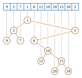
A treap with alphabetic key and numeric max heap order

The treap was first described by Raimund Seidel and Cecilia R. Aragon in 1989; ^{[1] [2]} its name is a portmanteau of tree and heap. It is a Cartesian tree in which each key is given a (randomly chosen) numeric priority. As with any binary search tree, the inorder traversal order of the nodes is the same as the sorted order of the keys. The structure of the tree is determined by the requirement that it be heap-ordered: that is, the priority number for any non-leaf node must be greater than or equal to the priority of its children. Thus, as with Cartesian trees more generally, the root node is the maximum-priority node, and its left and right subtrees are formed in the same manner from the subsequences of the sorted order to the left and right of that node.

An equivalent way of describing the treap is that it could be formed by inserting the nodes highest priority-first into a binary search tree without doing any rebalancing. Therefore, if the priorities are independent random numbers (from a distribution over a large enough space of possible priorities to ensure that two nodes are very unlikely to have the same priority) then the shape of a treap has the same probability distribution as the shape of a random binary search tree, a search tree formed by inserting the nodes without rebalancing in a randomly chosen insertion order. Because random binary search trees are known to have logarithmic height with high probability, the same is true for treaps. This mirrors the binary search tree argument that quicksort runs in expected ${\displaystyle O(n\log n)}$ time. If binary search trees are solutions to the dynamic problem version of sorting, then Treaps correspond specifically to dynamic quicksort where priorities guide pivot choices.

Aragon and Seidel also suggest assigning higher priorities to frequently accessed nodes, for instance by a process that, on each access, chooses a random number and replaces the priority of the node with that number if it is higher than the previous priority. This modification would cause the tree to lose its random shape; instead, frequently accessed nodes would be more likely to be near the root of the tree, causing searches for them to be faster.

Naor and Nissim ^[3] describe an application in maintaining authorization certificates in public-key cryptosystems.

Operations

Basic operations

Treaps support the following basic operations:

• To search for a given key value, apply a standard binary search algorithm in a binary search tree, ignoring the priorities.
• To insert a new key x into the treap, generate a random priority y for x. Binary search for x in the tree, and create a new node at the leaf position where the binary search determines a node for x should exist. Then, as long as x is not the root of the tree and has a larger priority number than its parent z, perform a tree rotation that reverses the parent-child relation between x and z.
• To delete a node x from the treap, if x is a leaf of the tree, simply remove it. If x has a single child z, remove x from the tree and make z be the child of the parent of x (or make z the root of the tree if x had no parent). Finally, if x has two children, swap its position in the tree with the position of its immediate successor z in the sorted order, resulting in one of the previous cases. In this final case, the swap may violate the heap-ordering property for z, so additional rotations may need to be performed to restore this property.

Building a treap

• To build a treap we can simply insert n values in the treap where each takes ${\displaystyle O(\log n)}$ time. Therefore a treap can be built in ${\displaystyle O(n\log n)}$ time from a list values.

Bulk operations

In addition to the single-element insert, delete and lookup operations, several fast "bulk" operations have been defined on treaps: union, intersection and set difference. These rely on two helper operations, split and join.

• To split a treap into two smaller treaps, those smaller than key x, and those larger than key x, insert x into the treap with maximum priority—larger than the priority of any node in the treap. After this insertion, x will be the root node of the treap, all values less than x will be found in the left subtreap, and all values greater than x will be found in the right subtreap. This costs as much as a single insertion into the treap.
• Joining two treaps that are the product of a former split, one can safely assume that the greatest value in the first treap is less than the smallest value in the second treap. Create a new node with value x, such that x is larger than this max-value in the first treap and smaller than the min-value in the second treap, assign it the minimum priority, then set its left child to the first heap and its right child to the second heap. Rotate as necessary to fix the heap order. After that, it will be a leaf node, and can easily be deleted. The result is one treap merged from the two original treaps. This is effectively "undoing" a split, and costs the same. More generally, the join operation can work on two treaps and a key with arbitrary priority (i.e., not necessary to be the highest).

Join performed on treaps ${\displaystyle T_{1}}$ and ${\displaystyle T_{2}}$. Right child of ${\displaystyle T_{1}}$ after the join is defined as a join of its former right child and ${\displaystyle T_{2}}$.

The join algorithm is as follows:

function join(L, k, R)     if prior(k, k(L)) and prior(k, k(R)) return Node(L, k, R)     if prior(k(L), k(R)) return Node(left(L), k(L), join(right(L), k, R))     return Node(join(L, k, left(R)), k(R), right(R))

To split ${\displaystyle T}$ by ${\displaystyle x}$, recursive split call is done to either left or right child of ${\displaystyle T}$.

The split algorithm is as follows:

function split(T, k)     if (T = nil) return (nil, false, nil)     (L, (m, c), R) = expose(T)     if (k = m) return (L, true, R)     if (k < m)          (L', b, R') = split(L, k)         return (L', b, join(R', m, R))     if (k > m)          (L', b, R') = split(R, k)         return (join(L, m, L'), b, R'))

The union of two treaps t₁ and t₂, representing sets A and B is a treap t that represents A ∪ B. The following recursive algorithm computes the union:

function union(t1, t2):     if t1 = nil:         return t2if t2 = nil:         return t1if priority(t1) < priority(t2):         swap t1 and t2     t<, t> ← split t2 on key(t1)     return join(union(left(t1), t<), key(t1),                     union(right(t1), t>))

Here, split is presumed to return two trees: one holding the keys less than its input key, one holding the greater keys. (The algorithm is non-destructive, but an in-place destructive version exists as well.)

The algorithm for intersection is similar, but requires the join helper routine. The complexity of each of union, intersection and difference is O(m log n/m) for treaps of sizes m and n, with m ≤ n. Moreover, since the recursive calls to union are independent of each other, they can be executed in parallel. ^[4]

Split and Union call Join but do not deal with the balancing criteria of treaps directly, such an implementation is usually called the "join-based" implementation.

Note that if hash values of keys are used as priorities and structurally equal nodes are merged already at construction, then each merged node will be a unique representation of a set of keys. Provided that there can only be one simultaneous root node representing a given set of keys, two sets can be tested for equality by pointer comparison, which is constant in time.

This technique can be used to enhance the merge algorithms to perform fast also when the difference between two sets is small. If input sets are equal, the union and intersection functions could break immediately returning one of the input sets as result, while the difference function should return the empty set.

Let d be the size of the symmetric difference. The modified merge algorithms will then also be bounded by O(d log n/d). ^{[5] [6]}

Randomized binary search tree

The randomized binary search tree, introduced by Martínez and Roura subsequently to the work of Aragon and Seidel on treaps, ^[7] stores the same nodes with the same random distribution of tree shape, but maintains different information within the nodes of the tree in order to maintain its randomized structure.

Rather than storing random priorities on each node, the randomized binary search tree stores a small integer at each node, the number of its descendants (counting itself as one); these numbers may be maintained during tree rotation operations at only a constant additional amount of time per rotation. When a key x is to be inserted into a tree that already has n nodes, the insertion algorithm chooses with probability 1/(n + 1) to place x as the new root of the tree, and otherwise, it calls the insertion procedure recursively to insert x within the left or right subtree (depending on whether its key is less than or greater than the root). The numbers of descendants are used by the algorithm to calculate the necessary probabilities for the random choices at each step. Placing x at the root of a subtree may be performed either as in the treap by inserting it at a leaf and then rotating it upwards, or by an alternative algorithm described by Martínez and Roura that splits the subtree into two pieces to be used as the left and right children of the new node.

The deletion procedure for a randomized binary search tree uses the same information per node as the insertion procedure, but unlike the insertion procedure, it only needs on average O(1) random decisions to join the two subtrees descending from the left and right children of the deleted node into a single tree. That is because the subtrees to be joined are on average at depth Θ(log n); joining two trees of size n and m needs Θ(log(n+m)) random choices on average. If the left or right subtree of the node to be deleted is empty, the join operation is trivial; otherwise, the left or right child of the deleted node is selected as the new subtree root with probability proportional to its number of descendants, and the join proceeds recursively.

Comparison

The information stored per node in the randomized binary tree is simpler than in a treap (a small integer rather than a high-precision random number), but it makes a greater number of calls to the random number generator (O(log n) calls per insertion or deletion rather than one call per insertion) and the insertion procedure is slightly more complicated due to the need to update the numbers of descendants per node. A minor technical difference is that, in a treap, there is a small probability of a collision (two keys getting the same priority), and in both cases, there will be statistical differences between a true random number generator and the pseudo-random number generator typically used on digital computers. However, in any case, the differences between the theoretical model of perfect random choices used to design the algorithm and the capabilities of actual random number generators are vanishingly small.

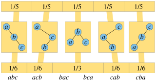
Although the treap and the randomized binary search tree both have the same random distribution of tree shapes after each update, the history of modifications to the trees performed by these two data structures over a sequence of insertion and deletion operations may be different. For instance, in a treap, if the three numbers 1, 2, and 3 are inserted in the order 1, 3, 2, and then the number 2 is deleted, the remaining two nodes will have the same parent-child relationship that they did prior to the insertion of the middle number. In a randomized binary search tree, the tree after the deletion is equally likely to be either of the two possible trees on its two nodes, independently of what the tree looked like prior to the insertion of the middle number.

Implicit treap

An implicit treap ^{[8] [ unreliable source? ]} is a simple variation of an ordinary treap which can be viewed as a dynamic array that supports the following operations in ${\displaystyle O(\log n)}$:

• Inserting an element in any position
• Removing an element from any position
• Finding sum, minimum or maximum element in a given range.
• Addition, painting in a given range
• Reversing elements in a given range

The idea behind an implicit treap is to use the array index as a key, but to not store it explicitly. Otherwise, an update (insertion/deletion) would result in changes of the keys in ${\displaystyle O(n)}$ nodes of the tree.

The key value (implicit key) of a node T is the number of nodes less than that node plus one. Note that such nodes can be present not only in its left subtree but also in left subtrees of its ancestors P, if T is in the right subtree of P.

Therefore we can quickly calculate the implicit key of the current node as we perform an operation by accumulating the sum of all nodes as we descend the tree. Note that this sum does not change when we visit the left subtree but it will increase by ${\displaystyle cnt(T\rightarrow L)+1}$ when we visit the right subtree.

The join algorithm for an implicit treap is as follows:

voidjoin(pitem&t,piteml,pitemr){if(!l||!r)t=l?l:r;elseif(l->prior>r->prior)join(l->r,l->r,r),t=l;elsejoin(r->l,l,r->l),t=r;upd_cnt(t);}

^[8] The split algorithm for an implicit treap is as follows:

voidsplit(pitemt,pitem&l,pitem&r,intkey,intadd=0){if(!t)returnvoid(l=r=0);intcur_key=add+cnt(t->l);//implicit keyif(key<=cur_key)split(t->l,l,t->l,key,add),r=t;elsesplit(t->r,t->r,r,key,add+1+cnt(t->l)),l=t;upd_cnt(t);}

^[8]

Operations

Insert element

To insert an element at position pos we divide the array into two subsections [0...pos-1] and [pos..sz] by calling the split function and we get two trees ${\displaystyle T1}$ and ${\displaystyle T2}$ . Then we merge ${\displaystyle T1}$ with the new node by calling the join function. Finally we call the join function to merge ${\displaystyle T1}$ and ${\displaystyle T2}$.

Delete element

We find the element to be deleted and perform a join on its children L and R. We then replace the element to be deleted with the tree that resulted from the join operation.

Find sum, minimum or maximum in a given range

To perform this calculation we will proceed as follows:

• First we will create an additional field F to store the value of the target function for the range represented by that node. we will create a function that calculates the value F based on the values of the L and R children of the node. We will call this target function at the end of all functions that modify the tree, i.e., split and join.
• Second we need to process a query for a given range [A..B]: We will call the split function twice and split the treap into ${\displaystyle T1}$ which contains ${\displaystyle \{1..A-1\}}$, ${\displaystyle T2}$ which contains ${\displaystyle \{A..B\}}$, and ${\displaystyle T3}$ which contains ${\displaystyle \{B+1..n\}}$. After the query is answered we will call the join function twice to restore the original treap.

Addition/painting in a given range

To perform this operation we will proceed as follows:

• We will create an extra field D which will contain the added value for the subtree. We will create a function push which will be used to propagate this change from a node to its children. We will call this function at the beginning of all functions which modify the tree, i.e., split and join so that after any changes made to the tree the information will not be lost.

Reverse in a given range

To show that the subtree of a given node needs to be reversed for each node we will create an extra boolean field R and set its value to true. To propagate this change we will swap the children of the node and set R to true for all of them.

See also

• Finger search

References

1. Aragon, Cecilia R.; Seidel, Raimund (1989), "Randomized Search Trees" (PDF), 30th Annual Symposium on Foundations of Computer Science, Washington, D.C.: IEEE Computer Society Press, pp. 540–545, doi:10.1109/SFCS.1989.63531, ISBN   0-8186-1982-1
2. Seidel, Raimund; Aragon, Cecilia R. (1996), "Randomized Search Trees", Algorithmica, 16 (4/5): 464–497, doi:10.1007/s004539900061
3. Naor, M.; Nissim, K. (April 2000), "Certificate revocation and certificate update" (PDF), IEEE Journal on Selected Areas in Communications, 18 (4): 561–570, doi:10.1109/49.839932, S2CID   13833836 ^{[ permanent dead link ]}.
4. Blelloch, Guy E.; Reid-Miller, Margaret (1998), "Fast set operations using treaps", Proceedings of the tenth annual ACM symposium on Parallel algorithms and architectures - SPAA '98, New York, NY, USA: ACM, pp. 16–26, doi:10.1145/277651.277660, ISBN   0-89791-989-0, S2CID   7342709 .
5. Liljenzin, Olle (2013). "Confluently Persistent Sets and Maps". arXiv: 1301.3388 . Bibcode:2013arXiv1301.3388L.{{cite journal}}: Cite journal requires |journal= (help)
6. Confluent Sets and Maps on GitHub
7. Martínez, Conrado; Roura, Salvador (1997), "Randomized binary search trees", Journal of the ACM, 45 (2): 288–323, doi: 10.1145/274787.274812 , S2CID   714621
8. "Treap - Competitive Programming Algorithms". cp-algorithms.com. Retrieved 2021-11-21.

External links

• Collection of treap references and info by Cecilia Aragon
• Open Data Structures - Section 7.2 - Treap: A Randomized Binary Search Tree, Pat Morin
• Animated treap
• Randomized binary search trees. Lecture notes from a course by Jeff Erickson at UIUC. Despite the title, this is primarily about treaps and skip lists; randomized binary search trees are mentioned only briefly.
• A high-performance key-value store based on treap by Junyi Sun
• VB6 implementation of treaps. Visual basic 6 implementation of treaps as a COM object.
• ActionScript3 implementation of a treap
• Pure Python and Cython in-memory treap and duptreap
• Treaps in C#. By Roy Clemmons
• Pure Go in-memory, immutable treaps
• Pure Go persistent treap key-value storage library