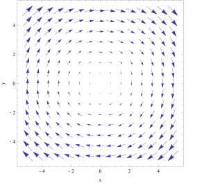
In vector calculus, the curl, also known as rotor, is a vector operator that describes the infinitesimal circulation of a vector field in three-dimensional Euclidean space. The curl at a point in the field is represented by a vector whose length and direction denote the magnitude and axis of the maximum circulation. The curl of a field is formally defined as the circulation density at each point of the field.

In geometry, a cube is a three-dimensional solid object bounded by six square faces, facets, or sides, with three meeting at each vertex. Viewed from a corner, it is a hexagon and its net is usually depicted as a cross.

In geometry, a tesseract is the four-dimensional analogue of the cube; the tesseract is to the cube as the cube is to the square. Just as the surface of the cube consists of six square faces, the hypersurface of the tesseract consists of eight cubical cells. The tesseract is one of the six convex regular 4-polytopes.

In geometry, a simplex is a generalization of the notion of a triangle or tetrahedron to arbitrary dimensions. The simplex is so-named because it represents the simplest possible polytope in any given dimension. For example,

In geometry, a hypercube is an n-dimensional analogue of a square and a cube. It is a closed, compact, convex figure whose 1-skeleton consists of groups of opposite parallel line segments aligned in each of the space's dimensions, perpendicular to each other and of the same length. A unit hypercube's longest diagonal in n dimensions is equal to .
In mathematics, Pascal's triangle is a triangular array of the binomial coefficients arising in probability theory, combinatorics, and algebra. In much of the Western world, it is named after the French mathematician Blaise Pascal, although other mathematicians studied it centuries before him in Persia, India, China, Germany, and Italy.

Perlin noise is a type of gradient noise developed by Ken Perlin in 1983. It has many uses, including but not limited to: procedurally generating terrain, applying pseudo-random changes to a variable, and assisting in the creation of image textures. It is most commonly implemented in two, three, or four dimensions, but can be defined for any number of dimensions.

In mathematics, a regular polytope is a polytope whose symmetry group acts transitively on its flags, thus giving it the highest degree of symmetry. All its elements or j-faces — cells, faces and so on — are also transitive on the symmetries of the polytope, and are regular polytopes of dimension ≤ n.

In geometry, a cross-polytope, hyperoctahedron, orthoplex, or cocube is a regular, convex polytope that exists in n-dimensional Euclidean space. A 2-dimensional cross-polytope is a square, a 3-dimensional cross-polytope is a regular octahedron, and a 4-dimensional cross-polytope is a 16-cell. Its facets are simplexes of the previous dimension, while the cross-polytope's vertex figure is another cross-polytope from the previous dimension.
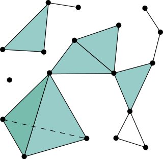
In combinatorics, an abstract simplicial complex (ASC), often called an abstract complex or just a complex, is a family of sets that is closed under taking subsets, i.e., every subset of a set in the family is also in the family. It is a purely combinatorial description of the geometric notion of a simplicial complex. For example, in a 2-dimensional simplicial complex, the sets in the family are the triangles, their edges, and their vertices.
In mathematics, a simplicial set is an object composed of simplices in a specific way. Simplicial sets are higher-dimensional generalizations of directed graphs, partially ordered sets and categories. Formally, a simplicial set may be defined as a contravariant functor from the simplex category to the category of sets. Simplicial sets were introduced in 1950 by Samuel Eilenberg and Joseph A. Zilber.
In algebraic topology, simplicial homology is the sequence of homology groups of a simplicial complex. It formalizes the idea of the number of holes of a given dimension in the complex. This generalizes the number of connected components.
In mathematics, the discrete Laplace operator is an analog of the continuous Laplace operator, defined so that it has meaning on a graph or a discrete grid. For the case of a finite-dimensional graph, the discrete Laplace operator is more commonly called the Laplacian matrix.
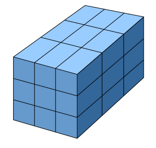
A regular grid is a tessellation of n-dimensional Euclidean space by congruent parallelotopes. Its opposite is irregular grid.

In geometry, demihypercubes (also called n-demicubes, n-hemicubes, and half measure polytopes) are a class of n-polytopes constructed from alternation of an n-hypercube, labeled as hγn for being half of the hypercube family, γn. Half of the vertices are deleted and new facets are formed. The 2n facets become 2n(n−1)-demicubes, and 2n(n−1)-simplex facets are formed in place of the deleted vertices.
Simplicial continuation, or piecewise linear continuation, is a one-parameter continuation method which is well suited to small to medium embedding spaces. The algorithm has been generalized to compute higher-dimensional manifolds by and.
In algebra, a multilinear polynomial is a multivariate polynomial that is linear in each of its variables separately, but not necessarily simultaneously. It is a polynomial in which no variable occurs to a power of 2 or higher; that is, each monomial is a constant times a product of distinct variables. For example f(x,y,z) = 3xy + 2.5 y - 7z is a multilinear polynomial of degree 2 whereas f(x,y,z) = x² +4y is not. The degree of a multilinear polynomial is the maximum number of distinct variables occurring in any monomial.

In geometry, the simplicial honeycomb is a dimensional infinite series of honeycombs, based on the affine Coxeter group symmetry. It is represented by a Coxeter-Dynkin diagram as a cyclic graph of n + 1 nodes with one node ringed. It is composed of n-simplex facets, along with all rectified n-simplices. It can be thought of as an n-dimensional hypercubic honeycomb that has been subdivided along all hyperplanes , then stretched along its main diagonal until the simplices on the ends of the hypercubes become regular. The vertex figure of an n-simplex honeycomb is an expanded n-simplex.

OpenSimplex noise is an n-dimensional gradient noise function that was developed in order to overcome the patent-related issues surrounding simplex noise, while likewise avoiding the visually-significant directional artifacts characteristic of Perlin noise.


