This article needs additional citations for verification .(May 2023) |
A low-pass filter is a filter that passes signals with a frequency lower than a selected cutoff frequency and attenuates signals with frequencies higher than the cutoff frequency. The exact frequency response of the filter depends on the filter design. The filter is sometimes called a high-cut filter, or treble-cut filter in audio applications. A low-pass filter is the complement of a high-pass filter.
Contents
- Examples
- Ideal and real filters
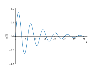
- Time response
- Step input response example
- Frequency response
- Difference equation through discrete time sampling
- Error analysis
- Discrete-time realization
- Simple infinite impulse response filter
- Finite impulse response
- Fourier transform
- Continuous-time realization
- Laplace notation
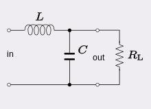
- Electronic low-pass filters
- First order
- Second order
- Second-Order Low-Pass Filter Standard Form
- Higher order passive filters
- Active electronic realization
- See also
- References
- External links
In optics, high-pass and low-pass may have different meanings, depending on whether referring to the frequency or wavelength of light, since these variables are inversely related. High-pass frequency filters would act as low-pass wavelength filters, and vice versa. For this reason, it is a good practice to refer to wavelength filters as short-pass and long-pass to avoid confusion, which would correspond to high-pass and low-pass frequencies. [1]
Low-pass filters exist in many different forms, including electronic circuits such as a hiss filter used in audio, anti-aliasing filters for conditioning signals before analog-to-digital conversion, digital filters for smoothing sets of data, acoustic barriers, blurring of images, and so on. The moving average operation used in fields such as finance is a particular kind of low-pass filter and can be analyzed with the same signal processing techniques as are used for other low-pass filters. Low-pass filters provide a smoother form of a signal, removing the short-term fluctuations and leaving the longer-term trend.
Filter designers will often use the low-pass form as a prototype filter. That is a filter with unity bandwidth and impedance. The desired filter is obtained from the prototype by scaling for the desired bandwidth and impedance and transforming into the desired bandform (that is, low-pass, high-pass, band-pass or band-stop).