Supply (economics)

Last updated
An example of a nonlinear supply curve Supply.gif
An example of a nonlinear supply curve

In economics, supply is the amount of a resource that firms, producers, labourers, providers of financial assets, or other economic agents are willing and able to provide to the marketplace or to an individual. Supply can be in produced goods, labour time, raw materials, or any other scarce or valuable object. Supply is often plotted graphically as a supply curve, with the price per unit on the vertical axis and quantity supplied as a function of price on the horizontal axis. This reversal of the usual position of the dependent variable and the independent variable is an unfortunate but standard convention.

Contents

The supply curve can be either for an individual seller or for the market as a whole, adding up the quantity supplied by all sellers. The quantity supplied is for a particular time period (e.g., the tons of steel a firm would supply in a year), but the units and time are often omitted in theoretical presentations.

In the goods market, supply is the amount of a product per unit of time that producers are willing to sell at various given prices when all other factors are held constant. In the labor market, the supply of labor is the amount of time per week, month, or year that individuals are willing to spend working, as a function of the wage rate.

In the economic and financial field, the money supply is the amount of highly liquid assets available in the money market, which is either determined or influenced by a country's monetary authority. This can vary based on which type of money supply one is discussing. M1 for example is commonly used to refer to narrow money, coins, cash, and other money equivalents that can be converted to currency nearly instantly. M2 by contrast includes all of M1 but also includes short-term deposits and certain types of market funds.

Supply schedule

A supply schedule is a table which shows how much one or more firms will be willing to supply at particular prices under the existing circumstances. [1] Some of the more important factors affecting supply are the good's own price, the prices of related goods, production costs, technology, the production function, and expectations of sellers.

Factors affecting supply

Innumerable factors and circumstances could affect a seller's willingness or ability to produce and sell a good. Some of the more common factors are:

Good's own price: The basic supply relationship is between the price of a good and the quantity supplied. According to the law of supply, keeping other factors constant, an increase in price results in an increase in quantity supplied. [2]
Prices of related goods: [2] For purposes of supply analysis related goods refer to goods from which inputs are derived to be used in the production of the primary good. For example, Spam is made from pork shoulders and ham. Both are derived from pigs. Therefore, pigs would be considered a related good to Spam. In this case the relationship would be negative or inverse. If the price of pigs goes up the supply of Spam would decrease (supply curve shifts left) because the cost of production would have increased. A related good may also be a good that can be produced with the firm's existing factors of production. For example, suppose that a firm produces leather belts, and that the firm's managers learn that leather pouches for smartphones are more profitable than belts. The firm might reduce its production of belts and begin production of cell phone pouches based on this information. Finally, a change in the price of a joint product will affect supply. For example, beef products and leather are joint products. If a company runs both a beef processing operation and a tannery an increase in the price of steaks would mean that more cattle are processed which would increase the supply of leather. [3]
Conditions of production: The most significant factor here is the state of technology. If there is a technological advancement in one good's production, the supply increases. Other variables may also affect production conditions. For instance, for agricultural goods, weather is crucial for it may affect the production outputs. [4] Economies of scale can also affect conditions of production.
Expectations: Sellers' concern for future market conditions can directly affect supply. [5] If the seller believes that the demand for his product will sharply increase in the foreseeable future the firm owner may immediately increase production in anticipation of future price increases. The supply curve would shift out. [6]
Price of inputs: Inputs include land, labor, energy and raw materials. [7] If the price of inputs increases the supply curve will shift left as sellers are less willing or able to sell goods at any given price. For example, if the price of electricity increased a seller may reduce his supply of his product because of the increased costs of production. [6] Fixed inputs can affect the price of inputs, and the scale of production can affect how much the fixed costs translate into the end price of the good.
Number of suppliers: The market supply curve is the horizontal summation of the individual supply curves. As more firms enter the industry, the market supply curve will shift out, driving down prices.
Government policies and regulations: Government intervention can have a significant effect on supply. [7] Government intervention can take many forms including environmental and health regulations, hour and wage laws, taxes, electrical and natural gas rates and zoning and land use regulations. [8]

This list is not exhaustive. All facts and circumstances that are relevant to a seller's willingness or ability to produce and sell goods can affect supply. [9] For example, if the forecast is for snow retail sellers will respond by increasing their stocks of snow sleds or skis or winter clothing or bread and milk.

Cases that violate the law of supply/ Exceptional cases to the law of supply

Agricultural products / Perishable goods: Due to their nature of having a short shelf life, immediately after harvest they are offered in the market for sale in large quantities during which prices are usually low. During dry season / planting season, it is the opposite.

Commodities produced in fixed amounts: For example some commodities which depend on the machine set up, in this case at different prices in the market the commodity may be offered in the same quantity.

Supply of labour in the market: The senior management/executive positions have high wages but work a few hours as compared to staff members who earn middle wage levels but work for the longest hours.[ according to whom? ]

Supply function and equation

Supply functions, then, may be classified according to the source from which they come: consumers or firms. Each type of supply function is now considered in turn. In so doing, the following notational conventions are employed: There are I produced goods, each defining a single industry, and J factors. The indices i = 1,…, I and J = 1,…, J run, respectively, over produced goods (industries) and factors. Let n index all goods by first listing produced goods and then factors so that n = 1,…, I, I + 1,…, I + J. The number of firms in industry i is written L i, and these firms are indexed by l = 1,…, L i. There are K consumers enumerated as k = 1,…, K. The variable represents the quantities of factor j consumed by consumer k. This person can have endowments of good j from to . If < then person k is a supplier of j. If the opposite is true, they are a consumer of j.

The supply function is the mathematical expression of the relationship between supply and those factors that affect the willingness and ability of a supplier to offer goods for sale. An example would be the curve implied by where is the price of the good and is the price of a related good. The semicolon means that the variables to the right are held constant when quantity supplied is plotted against the good's own price. The supply equation is the explicit mathematical expression of the functional relationship. A linear example is Here is the repository of all non-specified factors that affect supply for the product. The coefficient of is positive following the general rule that price and quantity supplied are directly related. is the price of a related good. Typically, its coefficient is negative because the related good is an input or a source of inputs.

Movements versus shifts

Movements along the curve occur only if there is a change in quantity supplied caused by a change in the good's own price. [10] A shift in the supply curve, referred to as a change in supply, occurs only if a non-price determinant of supply changes. [10] For example, if the price of an ingredient used to produce the good, a related good, were to increase, the supply curve would shift left. [11]

Inverse supply equation

By convention in the context of supply and demand graphs, economists graph the dependent variable (quantity) on the horizontal axis and the independent variable (price) on the vertical axis. The inverse supply equation is the equation written with the vertical-axis variable isolated on the left side: . As an example, if the supply equation is then the inverse supply equation would be . [12]

Marginal costs and short-run supply curve

A firm's short-run supply curve is the marginal cost curve above the shutdown point the short-run marginal cost curve (SRMC) above the minimum average variable cost. The portion of the SRMC below the shutdown point is not part of the supply curve because the firm is not producing any output. [13] The firm's long-run supply curve is that portion of the long-run marginal cost curve above the minimum of the long run average cost curve.

Shape of the short-run supply curve

The Law of Diminishing Marginal Returns (LDMR) shapes the SRMC curve. The LDMR states that as production increases eventually a point (the point of diminishing marginal returns) will be reached after which additional units of output resulting from fixed increments of the labor input will be successively smaller. That is, beyond the point of diminishing marginal returns the marginal product of labor will continually decrease and hence a continually higher selling price would be necessary to induce the firm to produce more and more output.

From firm to market supply curve

The market supply curve is the horizontal summation of firm supply curves. [14]

The market supply curve can be translated into an equation. For a factor j for example the market supply function is

where

and for all p > 0 and r > 0.

Note: not all assumptions that can be made for individual supply functions translate over to market supply functions directly.

The shape of the market supply curve

The law of supply dictates that all other things remaining equal, an increase in the price of the good in question results in an increase in quantity supplied. In other words, the supply curve slopes upwards. [15] However, there are exceptions to the law of supply. Not all supply curves slope upwards. [16]

Some heterodox economists, such as Steve Keen and Dirk Ehnts, dispute this theory of the supply curve, arguing that the supply curve for mass produced goods is often downward-sloping: as production increases, unit prices go down, and conversely, if demand is very low, unit prices go up. [17] [18] This corresponds to economies of scale.[ citation needed ]

Elasticity

The price elasticity of supply (PES) measures the responsiveness of quantity supplied to changes in price, as the percentage change in quantity supplied induced by a one percent change in price. It is calculated for discrete changes as and for smooth changes of differentiable supply functions as . Since supply is usually increasing in price, the price elasticity of supply is usually positive. For example, if the PES for a good is 0.67 a 1% rise in price will induce a two-thirds increase in quantity supplied.

Significant determinants include:

Complexity of production: Much depends on the complexity of the production process. Textile production is relatively simple. The labor is largely unskilled and production facilities are little more than buildings—no special structures are needed. Thus, the PES for textiles is elastic. On the other hand, the PES for specific types of motor vehicles is relatively inelastic. Auto manufacture is a multi-stage process that requires specialized equipment, skilled labor, a large suppliers network and large R&D costs.
Time to respond: The more time a producer has to respond to price changes the more elastic the supply. For example, a cotton farmer cannot immediately respond to an increase in the price of soybeans.
Excess capacity: A producer who has unused capacity can quickly respond to price changes in his market assuming that variable factors are readily available.
Inventories: A producer who has a supply of goods or available storage capacity can quickly respond to price changes.

Other elasticities can be calculated for non-price determinants of supply. For example, the percentage change the amount of the good supplied caused by a one percent increase in the price of a related good is an input elasticity of supply if the related good is an input in the production process.[ citation needed ] An example would be the change in the supply of cookies caused by a one percent increase in the price of sugar.

Elasticity along linear supply curves

The slope of a linear supply curve is constant; the elasticity is not. If the linear supply curve intersects the price axis, PES will be infinitely elastic at the point of intersection. [19] The coefficient of elasticity decreases as one moves "up" the curve. [19] However, all points on the supply curve will have a coefficient of elasticity greater than one. [20] If the linear supply curve intersects the quantity axis PES will equal zero at the point of intersection and will increase as one moves up the curve; [19] however, all points on the curve will have a coefficient of elasticity less than 1. If the linear supply curve intersects the origin PES equals one at the point of origin and along the curve.

Market structure and the supply curve

There is no such thing as a monopoly supply curve. [21] Perfect competition is the only market structure for which a supply function can be derived. In a perfectly competitive market the price is given by the marketplace from the point of view of the supplier; a manager of a competitive firm can state what quantity of goods will be supplied for any price by simply referring to the firm's marginal cost curve. To generate his supply function the seller could simply initially hypothetically set the price equal to zero and then incrementally increase the price; at each price he could calculate the hypothetical quantity supplied using the marginal cost curve. Following this process the manager could trace out the complete supply function. A monopolist cannot replicate this process because price is not imposed by the marketplace and hence is not an independent variable from the point of view of the firm; instead, the firm simultaneously chooses both the price and the quantity subject to the stipulation that together they form a point on the customers' demand curve. A change in demand can result in "changes in price with no changes in output, changes in output with no changes in price or both". [21] There is simply not a one-to-one relationship between price and quantity supplied. [22] There is no single function that relates price to quantity supplied.

Aggregate supply and demand in macroeconomics

Supply curve

Related Research Articles

<span class="mw-page-title-main">Microeconomics</span> Behavior of individuals and firms

Microeconomics is a branch of economics that studies the behavior of individuals and firms in making decisions regarding the allocation of scarce resources and the interactions among these individuals and firms. Microeconomics focuses on the study of individual markets, sectors, or industries as opposed to the national economy as a whole, which is studied in macroeconomics.

A monopoly, as described by Irving Fisher, is a market with the "absence of competition", creating a situation where a specific person or enterprise is the only supplier of a particular thing. This contrasts with a monopsony which relates to a single entity's control of a market to purchase a good or service, and with oligopoly and duopoly which consists of a few sellers dominating a market. Monopolies are thus characterised by a lack of economic competition to produce the good or service, a lack of viable substitute goods, and the possibility of a high monopoly price well above the seller's marginal cost that leads to a high monopoly profit. The verb monopolise or monopolize refers to the process by which a company gains the ability to raise prices or exclude competitors. In economics, a monopoly is a single seller. In law, a monopoly is a business entity that has significant market power, that is, the power to charge overly high prices, which is associated with a decrease in social surplus. Although monopolies may be big businesses, size is not a characteristic of a monopoly. A small business may still have the power to raise prices in a small industry.

In economics, specifically general equilibrium theory, a perfect market, also known as an atomistic market, is defined by several idealizing conditions, collectively called perfect competition, or atomistic competition. In theoretical models where conditions of perfect competition hold, it has been demonstrated that a market will reach an equilibrium in which the quantity supplied for every product or service, including labor, equals the quantity demanded at the current price. This equilibrium would be a Pareto optimum.

<span class="mw-page-title-main">Supply and demand</span> Economic model of price determination in a market

In microeconomics, supply and demand is an economic model of price determination in a market. It postulates that, holding all else equal, in a competitive market, the unit price for a particular good or other traded item such as labor or liquid financial assets, will vary until it settles at a point where the quantity demanded will equal the quantity supplied, resulting in an economic equilibrium for price and quantity transacted. The concept of supply and demand forms the theoretical basis of modern economics.

<span class="mw-page-title-main">Deadweight loss</span> Measure of lost economic efficiency

In economics, deadweight loss is the difference in production and consumption of any given product or service including government tax. The presence of deadweight loss is most commonly identified when the quantity produced relative to the amount consumed differs in regards to the optimal concentration of surplus. This difference in the amount reflects the quantity that is not being utilized or consumed and thus resulting in a loss. This "deadweight loss" is therefore attributed to both producers and consumers because neither one of them benefits from the surplus of the overall production.

<span class="mw-page-title-main">Profit maximization</span> Process to determine the highest profits for a firm

In economics, profit maximization is the short run or long run process by which a firm may determine the price, input and output levels that will lead to the highest possible total profit. In neoclassical economics, which is currently the mainstream approach to microeconomics, the firm is assumed to be a "rational agent" which wants to maximize its total profit, which is the difference between its total revenue and its total cost.

In economics, elasticity measures the responsiveness of one economic variable to a change in another. If the price elasticity of the demand of something is -2, a 10% increase in price causes the quantity demanded to fall by 20%. Elasticity in economics provides an understanding of changes in the behavior of the buyers and sellers with price changes. There are two types of elasticity for demand and supply, one is inelastic demand and supply and the other one is elastic demand and supply.

A good's price elasticity of demand is a measure of how sensitive the quantity demanded is to its price. When the price rises, quantity demanded falls for almost any good, but it falls more for some than for others. The price elasticity gives the percentage change in quantity demanded when there is a one percent increase in price, holding everything else constant. If the elasticity is −2, that means a one percent price rise leads to a two percent decline in quantity demanded. Other elasticities measure how the quantity demanded changes with other variables.

In economics, the marginal cost is the change in the total cost that arises when the quantity produced is increased, i.e. the cost of producing additional quantity. In some contexts, it refers to an increment of one unit of output, and in others it refers to the rate of change of total cost as output is increased by an infinitesimal amount. As Figure 1 shows, the marginal cost is measured in dollars per unit, whereas total cost is in dollars, and the marginal cost is the slope of the total cost, the rate at which it increases with output. Marginal cost is different from average cost, which is the total cost divided by the number of units produced.

<span class="mw-page-title-main">Substitute good</span> Economics concept of goods considered interchangeable

In microeconomics, substitute goods are two goods that can be used for the same purpose by consumers. That is, a consumer perceives both goods as similar or comparable, so that having more of one good causes the consumer to desire less of the other good. Contrary to complementary goods and independent goods, substitute goods may replace each other in use due to changing economic conditions. An example of substitute goods is Coca-Cola and Pepsi; the interchangeable aspect of these goods is due to the similarity of the purpose they serve, i.e. fulfilling customers' desire for a soft drink. These types of substitutes can be referred to as close substitutes.

Managerial economics is a branch of economics involving the application of economic methods in the organizational decision-making process. Economics is the study of the production, distribution, and consumption of goods and services. Managerial economics involves the use of economic theories and principles to make decisions regarding the allocation of scarce resources. It guides managers in making decisions relating to the company's customers, competitors, suppliers, and internal operations.

<span class="mw-page-title-main">Price elasticity of supply</span> Measure in economics

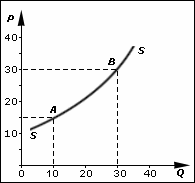
The price elasticity of supply is a measure used in economics to show the responsiveness, or elasticity, of the quantity supplied of a good or service to a change in its price. Price elasticity of supply, in application, is the percentage change of the quantity supplied resulting from a 1% change in price. Alternatively, PES is the percentage change in the quantity supplied divided by the percentage change in price.

<span class="mw-page-title-main">Law of demand</span> Fundamental principle in microeconomics

In microeconomics, the law of demand is a fundamental principle which states that there is an inverse relationship between price and quantity demanded. In other words, "conditional on all else being equal, as the price of a good increases (↑), quantity demanded will decrease (↓); conversely, as the price of a good decreases (↓), quantity demanded will increase (↑)". Alfred Marshall worded this as: "When we say that a person's demand for anything increases, we mean that he will buy more of it than he would before at the same price, and that he will buy as much of it as before at a higher price". The law of demand, however, only makes a qualitative statement in the sense that it describes the direction of change in the amount of quantity demanded but not the magnitude of change.

<span class="mw-page-title-main">Demand curve</span> Graph of how much of something a consumer would buy at a certain price

A demand curve is a graph depicting the inverse demand function, a relationship between the price of a certain commodity and the quantity of that commodity that is demanded at that price. Demand curves can be used either for the price-quantity relationship for an individual consumer, or for all consumers in a particular market.

<span class="mw-page-title-main">Marginal revenue</span> Additional total revenue generated by increasing product sales by 1 unit

Marginal revenue is a central concept in microeconomics that describes the additional total revenue generated by increasing product sales by 1 unit. Marginal revenue is the increase in revenue from the sale of one additional unit of product, i.e., the revenue from the sale of the last unit of product. It can be positive or negative. Marginal revenue is an important concept in vendor analysis. To derive the value of marginal revenue, it is required to examine the difference between the aggregate benefits a firm received from the quantity of a good and service produced last period and the current period with one extra unit increase in the rate of production. Marginal revenue is a fundamental tool for economic decision making within a firm's setting, together with marginal cost to be considered.

In economics, a cost curve is a graph of the costs of production as a function of total quantity produced. In a free market economy, productively efficient firms optimize their production process by minimizing cost consistent with each possible level of production, and the result is a cost curve. Profit-maximizing firms use cost curves to decide output quantities. There are various types of cost curves, all related to each other, including total and average cost curves; marginal cost curves, which are equal to the differential of the total cost curves; and variable cost curves. Some are applicable to the short run, others to the long run.

In economics, demand is the quantity of a good that consumers are willing and able to purchase at various prices during a given time. The relationship between price and quantity demand is also called the demand curve. Demand for a specific item is a function of an item's perceived necessity, price, perceived quality, convenience, available alternatives, purchasers' disposable income and tastes, and many other options.

Total revenue is the total receipts a seller can obtain from selling goods or services to buyers. It can be written as P × Q, which is the price of the goods multiplied by the quantity of the sold goods.

<span class="mw-page-title-main">Factor market</span> In economics, a market where resources used in the production process are bought and sold

In economics, a factor market is a market where factors of production are bought and sold. Factor markets allocate factors of production, including land, labour and capital, and distribute income to the owners of productive resources, such as wages, rents, etc.

<span class="mw-page-title-main">Monopoly price</span> Aspect of monopolistic markets

In microeconomics, a monopoly price is set by a monopoly. A monopoly occurs when a firm lacks any viable competition and is the sole producer of the industry's product. Because a monopoly faces no competition, it has absolute market power and can set a price above the firm's marginal cost.

References

  1. Mankiw, N. Gregory (1998). Principles of Economics, Wall Street Journal Edition. Dryden Press, San Diego. pp. 71–73. ISBN   0-03-098238-3.
  2. 1 2 Melvin & Boyes, Microeconomics 5th ed. (Houghton Mifflin 2002)
  3. Ayers & Collins, Microeconomics (Pearson 2003) at 66.
  4. Rosen, Harvey (2005). Public Finance, p. 545. McGraw-Hill/Irwin, New York. ISBN   0-07-287648-4.
  5. Goodwin, N, Nelson, J; Ackerman, F & Weissskopf, T: Microeconomics in Context 2d ed. Page 83 Sharpe 2009
  6. 1 2 Goodwin, Nelson, Ackerman, & Weissskopf, Microeconomics in Context 2d ed. (Sharpe 2009) at 83.
  7. 1 2 Samuelson & Nordhaus, Microeconomics, 17th ed. (McGraw-Hill 2001), p. 53.
  8. Samuelson & Nordhaus, Microeconomics, 17th ed. (McGraw-Hill 2001) at 56
  9. Colander, David C. Microeconomics 7th ed. Page 90. McGraw-Hill 2008.
  10. 1 2 Melvin & Boyes, Microeconomics 5th ed. (Houghton Mifflin 2002) at 60.
  11. Melvin & Boyes, Microeconomics 5th ed. (Houghton Mifflin 2002) at 56–62.
  12. Perloff, J. (2008). Microeconomics Theory & Applications with Calculus. Pearson. p. 56.
  13. Technically the short-run supply curve is a discontinuous function which begins at the origin then tracks the y axis until reaching a point level with the shutdown point.
  14. Melvin & Boyes, Microeconomics 5th ed. (Houghton Mifflin 2002) at 56.
  15. Mas-Colell, A., Whinston, M. Green, J.: Principles of Microeconomics. Oxford University Press., pg 138. 1995.
  16. Perloff, Microeconomics Theory & Applications with Calculus (Pearson 2008) at 19. Png, Managerial Economics (Blackwell 1999)
  17. Ehnts, Dirk (April 29, 2019). "The problem with the supply curve". econoblog101. Retrieved October 18, 2022.
  18. Keen, Steve (2011). "Chapter 5: The price of everything and the value of nothing". Debunking Economics: The Naked Emperor Dethroned? . Zed Books. ISBN   978-1848139923.
  19. 1 2 3 Colander, David C. (2008). Microeconomics (7th ed.). McGraw-Hill. pp. 132–133
  20. Colander p. 135.
  21. 1 2 Pindyck & Rubinfeld, Microeconomics 5th ed. (Prentice-Hall 2001) at 335.
  22. Pindyck & Rubinfeld, Microeconomics 5th ed. (Prentice-Hall 2001) at 336.