Linear prediction is a mathematical operation where future values of a discrete-time signal are estimated as a linear function of previous samples.
An adaptive filter is a system with a linear filter that has a transfer function controlled by variable parameters and a means to adjust those parameters according to an optimization algorithm. Because of the complexity of the optimization algorithms, almost all adaptive filters are digital filters. Adaptive filters are required for some applications because some parameters of the desired processing operation are not known in advance or are changing. The closed loop adaptive filter uses feedback in the form of an error signal to refine its transfer function.
Filter design is the process of designing a signal processing filter that satisfies a set of requirements, some of which may be conflicting. The purpose is to find a realization of the filter that meets each of the requirements to an acceptable degree.

In statistics and control theory, Kalman filtering is an algorithm that uses a series of measurements observed over time, including statistical noise and other inaccuracies, to produce estimates of unknown variables that tend to be more accurate than those based on a single measurement, by estimating a joint probability distribution over the variables for each time-step. The filter is constructed as a mean squared error minimiser, but an alternative derivation of the filter is also provided showing how the filter relates to maximum likelihood statistics. The filter is named after Rudolf E. Kálmán.
In signal processing, the Wiener filter is a filter used to produce an estimate of a desired or target random process by linear time-invariant (LTI) filtering of an observed noisy process, assuming known stationary signal and noise spectra, and additive noise. The Wiener filter minimizes the mean square error between the estimated random process and the desired process.
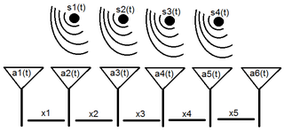
Array processing is a wide area of research in the field of signal processing that extends from the simplest form of 1 dimensional line arrays to 2 and 3 dimensional array geometries. Array structure can be defined as a set of sensors that are spatially separated, e.g. radio antenna and seismic arrays. The sensors used for a specific problem may vary widely, for example microphones, accelerometers and telescopes. However, many similarities exist, the most fundamental of which may be an assumption of wave propagation. Wave propagation means there is a systemic relationship between the signal received on spatially separated sensors. By creating a physical model of the wave propagation, or in machine learning applications a training data set, the relationships between the signals received on spatially separated sensors can be leveraged for many applications.
Estimation theory is a branch of statistics that deals with estimating the values of parameters based on measured empirical data that has a random component. The parameters describe an underlying physical setting in such a way that their value affects the distribution of the measured data. An estimator attempts to approximate the unknown parameters using the measurements. In estimation theory, two approaches are generally considered:
Least mean squares (LMS) algorithms are a class of adaptive filter used to mimic a desired filter by finding the filter coefficients that relate to producing the least mean square of the error signal. It is a stochastic gradient descent method in that the filter is only adapted based on the error at the current time. It was invented in 1960 by Stanford University professor Bernard Widrow and his first Ph.D. student, Ted Hoff, based on their research in single-layer neural networks (ADALINE). Specifically, they used gradient descent to train ADALINE to recognize patterns, and called the algorithm "delta rule". They then applied the rule to filters, resulting in the LMS algorithm.
Recursive least squares (RLS) is an adaptive filter algorithm that recursively finds the coefficients that minimize a weighted linear least squares cost function relating to the input signals. This approach is in contrast to other algorithms such as the least mean squares (LMS) that aim to reduce the mean square error. In the derivation of the RLS, the input signals are considered deterministic, while for the LMS and similar algorithms they are considered stochastic. Compared to most of its competitors, the RLS exhibits extremely fast convergence. However, this benefit comes at the cost of high computational complexity.
In machine learning, kernel machines are a class of algorithms for pattern analysis, whose best known member is the support-vector machine (SVM). These methods involve using linear classifiers to solve nonlinear problems. The general task of pattern analysis is to find and study general types of relations in datasets. For many algorithms that solve these tasks, the data in raw representation have to be explicitly transformed into feature vector representations via a user-specified feature map: in contrast, kernel methods require only a user-specified kernel, i.e., a similarity function over all pairs of data points computed using inner products. The feature map in kernel machines is infinite dimensional but only requires a finite dimensional matrix from user-input according to the Representer theorem. Kernel machines are slow to compute for datasets larger than a couple of thousand examples without parallel processing.
In wireless communications, channel state information (CSI) is the known channel properties of a communication link. This information describes how a signal propagates from the transmitter to the receiver and represents the combined effect of, for example, scattering, fading, and power decay with distance. The method is called channel estimation. The CSI makes it possible to adapt transmissions to current channel conditions, which is crucial for achieving reliable communication with high data rates in multiantenna systems.

Space-time adaptive processing (STAP) is a signal processing technique most commonly used in radar systems. It involves adaptive array processing algorithms to aid in target detection. Radar signal processing benefits from STAP in areas where interference is a problem. Through careful application of STAP, it is possible to achieve order-of-magnitude sensitivity improvements in target detection.
Blind equalization is a digital signal processing technique in which the transmitted signal is inferred (equalized) from the received signal, while making use only of the transmitted signal statistics. Hence, the use of the word blind in the name.
The multidelay block frequency domain adaptive filter (MDF) algorithm is a block-based frequency domain implementation of the (normalised) Least mean squares filter (LMS) algorithm.
Precoding is a generalization of beamforming to support multi-stream transmission in multi-antenna wireless communications. In conventional single-stream beamforming, the same signal is emitted from each of the transmit antennas with appropriate weighting such that the signal power is maximized at the receiver output. When the receiver has multiple antennas, single-stream beamforming cannot simultaneously maximize the signal level at all of the receive antennas. In order to maximize the throughput in multiple receive antenna systems, multi-stream transmission is generally required.
Zero-forcing precoding is a method of spatial signal processing by which a multiple antenna transmitter can null the multiuser interference in a multi-user MIMO wireless communication system. When the channel state information is perfectly known at the transmitter, the zero-forcing precoder is given by the pseudo-inverse of the channel matrix. Zero-forcing has been used in LTE mobile networks.

In probability theory and statistics, the generalized chi-squared distribution is the distribution of a quadratic form of a multinormal variable, or a linear combination of different normal variables and squares of normal variables. Equivalently, it is also a linear sum of independent noncentral chi-square variables and a normal variable. There are several other such generalizations for which the same term is sometimes used; some of them are special cases of the family discussed here, for example the gamma distribution.
In signal processing, a kernel adaptive filter is a type of nonlinear adaptive filter. An adaptive filter is a filter that adapts its transfer function to changes in signal properties over time by minimizing an error or loss function that characterizes how far the filter deviates from ideal behavior. The adaptation process is based on learning from a sequence of signal samples and is thus an online algorithm. A nonlinear adaptive filter is one in which the transfer function is nonlinear.
A two-dimensional (2D) adaptive filter is very much like a one-dimensional adaptive filter in that it is a linear system whose parameters are adaptively updated throughout the process, according to some optimization approach. The main difference between 1D and 2D adaptive filters is that the former usually take as inputs signals with respect to time, what implies in causality constraints, while the latter handles signals with 2 dimensions, like x-y coordinates in the space domain, which are usually non-causal. Moreover, just like 1D filters, most 2D adaptive filters are digital filters, because of the complex and iterative nature of the algorithms.
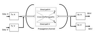
XPIC, or cross-polarization interference cancelling technology, is an algorithm to suppress mutual interference between two received streams in a Polarization-division multiplexing communication system.


