Backpropagation through time

Last updated

Backpropagation through time (BPTT) is a gradient-based technique for training certain types of recurrent neural networks. It can be used to train Elman networks. The algorithm was independently derived by numerous researchers. [1] [2] [3]

Contents

Algorithm

BPTT unfolds a recurrent neural network through time. Unfold through time.png
BPTT unfolds a recurrent neural network through time.

The training data for a recurrent neural network is an ordered sequence of input-output pairs, . An initial value must be specified for the hidden state . Typically, a vector of all zeros is used for this purpose.

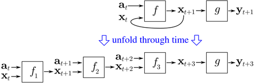
BPTT begins by unfolding a recurrent neural network in time. The unfolded network contains inputs and outputs, but every copy of the network shares the same parameters. Then the backpropagation algorithm is used to find the gradient of the cost with respect to all the network parameters.

Consider an example of a neural network that contains a recurrent layer and a feedforward layer . There are different ways to define the training cost, but the aggregated cost is always the average of the costs of each of the time steps. The cost of each time step can be computed separately. The figure above shows how the cost at time can be computed, by unfolding the recurrent layer for three time steps and adding the feedforward layer . Each instance of in the unfolded network shares the same parameters. Thus the weight updates in each instance () are summed together.

Pseudocode

Pseudocode for a truncated version of BPTT, where the training data contains input-output pairs, but the network is unfolded for time steps:

Back_Propagation_Through_Time(a, y)   // a[t] is the input at time t. y[t] is the output     Unfold the network to contain k instances of fdo until stopping criterion is met:         x := the zero-magnitude vector // x is the current context         for t from 0 to n − k do      // t is time. n is the length of the training sequence             Set the network inputs to x, a[t], a[t+1], ..., a[t+k−1]             p := forward-propagate the inputs over the whole unfolded network             e := y[t+k] − p;           // error = target − prediction             Back-propagate the error, e, back across the whole unfolded network             Sum the weight changes in the k instances of f together.             Update all the weights in f and g.             x := f(x, a[t]);           // compute the context for the next time-step

Advantages

BPTT tends to be significantly faster for training recurrent neural networks than general-purpose optimization techniques such as evolutionary optimization. [4]

Disadvantages

BPTT has difficulty with local optima. With recurrent neural networks, local optima are a much more significant problem than with feed-forward neural networks. [5] The recurrent feedback in such networks tends to create chaotic responses in the error surface which cause local optima to occur frequently, and in poor locations on the error surface.

See also

Related Research Articles

<span class="mw-page-title-main">Artificial neural network</span> Computational model used in machine learning, based on connected, hierarchical functions

Artificial neural networks are a branch of machine learning models that are built using principles of neuronal organization discovered by connectionism in the biological neural networks constituting animal brains.

<span class="mw-page-title-main">Perceptron</span> Algorithm for supervised learning of binary classifiers

In machine learning, the perceptron is an algorithm for supervised learning of binary classifiers. A binary classifier is a function which can decide whether or not an input, represented by a vector of numbers, belongs to some specific class. It is a type of linear classifier, i.e. a classification algorithm that makes its predictions based on a linear predictor function combining a set of weights with the feature vector.

Hebbian theory is a neuropsychological theory claiming that an increase in synaptic efficacy arises from a presynaptic cell's repeated and persistent stimulation of a postsynaptic cell. It is an attempt to explain synaptic plasticity, the adaptation of brain neurons during the learning process. It was introduced by Donald Hebb in his 1949 book The Organization of Behavior. The theory is also called Hebb's rule, Hebb's postulate, and cell assembly theory. Hebb states it as follows:

Let us assume that the persistence or repetition of a reverberatory activity tends to induce lasting cellular changes that add to its stability. ... When an axon of cell A is near enough to excite a cell B and repeatedly or persistently takes part in firing it, some growth process or metabolic change takes place in one or both cells such that A’s efficiency, as one of the cells firing B, is increased.

Multi-task learning (MTL) is a subfield of machine learning in which multiple learning tasks are solved at the same time, while exploiting commonalities and differences across tasks. This can result in improved learning efficiency and prediction accuracy for the task-specific models, when compared to training the models separately. Early versions of MTL were called "hints".

<span class="mw-page-title-main">Backpropagation</span> Optimization algorithm for artificial neural networks

As a machine-learning algorithm, backpropagation performs a backward pass to adjust a neural network model's parameters, aiming to minimize the mean squared error (MSE). In a multi-layered network, backpropagation uses the following steps:

  1. Propagate training data through the model from input to predicted output by computing the successive hidden layers' outputs and finally the final layer's output.
  2. Adjust the model weights to reduce the error relative to the weights.
    1. The error is typically the squared difference between prediction and target.
    2. For each weight, the slope or derivative of the error is found, and the weight adjusted by a negative multiple of this derivative, so as to go downslope toward the minimum-error configuration.
    3. This derivative is easy to calculate for final layer weights, and possible to calculate for one layer given the next layer's derivatives. Starting at the end, then, the derivatives are calculated layer by layer toward the beginning -- thus "backpropagation".
  3. Repeatedly update the weights until they converge or the model has undergone enough iterations.
<span class="mw-page-title-main">Recurrent neural network</span> Computational model used in machine learning

A recurrent neural network (RNN) is one of the two broad types of artificial neural network, characterized by direction of the flow of information between its layers. In contrast to uni-directional feedforward neural network, it is a bi-directional artificial neural network, meaning that it allows the output from some nodes to affect subsequent input to the same nodes. Their ability to use internal state (memory) to process arbitrary sequences of inputs makes them applicable to tasks such as unsegmented, connected handwriting recognition or speech recognition. The term "recurrent neural network" is used to refer to the class of networks with an infinite impulse response, whereas "convolutional neural network" refers to the class of finite impulse response. Both classes of networks exhibit temporal dynamic behavior. A finite impulse recurrent network is a directed acyclic graph that can be unrolled and replaced with a strictly feedforward neural network, while an infinite impulse recurrent network is a directed cyclic graph that can not be unrolled.

<span class="mw-page-title-main">Feedforward neural network</span> One of two broad types of artificial neural network

A feedforward neural network (FNN) is one of the two broad types of artificial neural network, characterized by direction of the flow of information between its layers. Its flow is uni-directional, meaning that the information in the model flows in only one direction—forward—from the input nodes, through the hidden nodes and to the output nodes, without any cycles or loops, in contrast to recurrent neural networks, which have a bi-directional flow. Modern feedforward networks are trained using the backpropagation method and are colloquially referred to as the "vanilla" neural networks.

<span class="mw-page-title-main">Multilayer perceptron</span> Type of feedforward neural network

A multilayer perceptron (MLP) is a misnomer for a modern feedforward artificial neural network, consisting of fully connected neurons with a nonlinear kind of activation function, organized in at least three layers, notable for being able to distinguish data that is not linearly separable. It is a misnomer because the original perceptron used a Heaviside step function, instead of a nonlinear kind of activation function.

<span class="mw-page-title-main">Kernel method</span> Class of algorithms for pattern analysis

In machine learning, kernel machines are a class of algorithms for pattern analysis, whose best known member is the support-vector machine (SVM). These methods involve using linear classifiers to solve nonlinear problems. The general task of pattern analysis is to find and study general types of relations in datasets. For many algorithms that solve these tasks, the data in raw representation have to be explicitly transformed into feature vector representations via a user-specified feature map: in contrast, kernel methods require only a user-specified kernel, i.e., a similarity function over all pairs of data points computed using inner products. The feature map in kernel machines is infinite dimensional but only requires a finite dimensional matrix from user-input according to the Representer theorem. Kernel machines are slow to compute for datasets larger than a couple of thousand examples without parallel processing.

<span class="mw-page-title-main">Quantum neural network</span> Quantum Mechanics in Neural Networks

Quantum neural networks are computational neural network models which are based on the principles of quantum mechanics. The first ideas on quantum neural computation were published independently in 1995 by Subhash Kak and Ron Chrisley, engaging with the theory of quantum mind, which posits that quantum effects play a role in cognitive function. However, typical research in quantum neural networks involves combining classical artificial neural network models with the advantages of quantum information in order to develop more efficient algorithms. One important motivation for these investigations is the difficulty to train classical neural networks, especially in big data applications. The hope is that features of quantum computing such as quantum parallelism or the effects of interference and entanglement can be used as resources. Since the technological implementation of a quantum computer is still in a premature stage, such quantum neural network models are mostly theoretical proposals that await their full implementation in physical experiments.

<span class="mw-page-title-main">ADALINE</span> Early single-layer artificial neural network

ADALINE is an early single-layer artificial neural network and the name of the physical device that implemented this network. The network uses memistors. It was developed by professor Bernard Widrow and his doctoral student Ted Hoff at Stanford University in 1960. It is based on the perceptron. It consists of a weight, a bias and a summation function.

Oja's learning rule, or simply Oja's rule, named after Finnish computer scientist Erkki Oja, is a model of how neurons in the brain or in artificial neural networks change connection strength, or learn, over time. It is a modification of the standard Hebb's Rule that, through multiplicative normalization, solves all stability problems and generates an algorithm for principal components analysis. This is a computational form of an effect which is believed to happen in biological neurons.

In the field of mathematical modeling, a radial basis function network is an artificial neural network that uses radial basis functions as activation functions. The output of the network is a linear combination of radial basis functions of the inputs and neuron parameters. Radial basis function networks have many uses, including function approximation, time series prediction, classification, and system control. They were first formulated in a 1988 paper by Broomhead and Lowe, both researchers at the Royal Signals and Radar Establishment.

The generalized Hebbian algorithm (GHA), also known in the literature as Sanger's rule, is a linear feedforward neural network model for unsupervised learning with applications primarily in principal components analysis. First defined in 1989, it is similar to Oja's rule in its formulation and stability, except it can be applied to networks with multiple outputs. The name originates because of the similarity between the algorithm and a hypothesis made by Donald Hebb about the way in which synaptic strengths in the brain are modified in response to experience, i.e., that changes are proportional to the correlation between the firing of pre- and post-synaptic neurons.

There are many types of artificial neural networks (ANN).

<span class="mw-page-title-main">Vanishing gradient problem</span> Machine learning model training problem

In machine learning, the vanishing gradient problem is encountered when training artificial neural networks with gradient-based learning methods and backpropagation. In such methods, during each iteration of training each of the neural networks weights receives an update proportional to the partial derivative of the error function with respect to the current weight. The problem is that in some cases, the gradient will be vanishingly small, effectively preventing the weight from changing its value. In the worst case, this may completely stop the neural network from further training. As one example of the problem cause, traditional activation functions such as the hyperbolic tangent function have gradients in the range (0,1], and backpropagation computes gradients by the chain rule. This has the effect of multiplying n of these small numbers to compute gradients of the early layers in an n-layer network, meaning that the gradient decreases exponentially with n while the early layers train very slowly.

<span class="mw-page-title-main">Extreme learning machine</span> Type of artificial neural network

Extreme learning machines are feedforward neural networks for classification, regression, clustering, sparse approximation, compression and feature learning with a single layer or multiple layers of hidden nodes, where the parameters of hidden nodes need to be tuned. These hidden nodes can be randomly assigned and never updated, or can be inherited from their ancestors without being changed. In most cases, the output weights of hidden nodes are usually learned in a single step, which essentially amounts to learning a linear model.

<span class="mw-page-title-main">Residual neural network</span> Deep learning method

A Residual Neural Network is a deep learning model in which the weight layers learn residual functions with reference to the layer inputs. A Residual Network is a network with skip connections that perform identity mappings, merged with the layer outputs by addition. It behaves like a Highway Network whose gates are opened through strongly positive bias weights. This enables deep learning models with tens or hundreds of layers to train easily and approach better accuracy when going deeper. The identity skip connections, often referred to as "residual connections", are also used in the 1997 LSTM networks, Transformer models, the AlphaGo Zero system, the AlphaStar system, and the AlphaFold system.

An artificial neural network (ANN) combines biological principles with advanced statistics to solve problems in domains such as pattern recognition and game-play. ANNs adopt the basic model of neuron analogues connected to each other in a variety of ways.

In the study of artificial neural networks (ANNs), the neural tangent kernel (NTK) is a kernel that describes the evolution of deep artificial neural networks during their training by gradient descent. It allows ANNs to be studied using theoretical tools from kernel methods.

References

  1. Mozer, M. C. (1995). "A Focused Backpropagation Algorithm for Temporal Pattern Recognition". In Chauvin, Y.; Rumelhart, D. (eds.). Backpropagation: Theory, architectures, and applications. pp. 137–169. Retrieved 2017-08-21.{{cite book}}: |website= ignored (help)
  2. Robinson, A. J. & Fallside, F. (1987). The utility driven dynamic error propagation network (Technical report). Cambridge University, Engineering Department. CUED/F-INFENG/TR.1.
  3. Werbos, Paul J. (1988). "Generalization of backpropagation with application to a recurrent gas market model". Neural Networks. 1 (4): 339–356. doi:10.1016/0893-6080(88)90007-x.
  4. Sjöberg, Jonas; Zhang, Qinghua; Ljung, Lennart; Benveniste, Albert; Delyon, Bernard; Glorennec, Pierre-Yves; Hjalmarsson, Håkan; Juditsky, Anatoli (1995). "Nonlinear black-box modeling in system identification: a unified overview". Automatica. 31 (12): 1691–1724. CiteSeerX   10.1.1.27.81 . doi:10.1016/0005-1098(95)00120-8.
  5. M.P. Cuéllar and M. Delgado and M.C. Pegalajar (2006). "An Application of Non-Linear Programming to Train Recurrent Neural Networks in Time Series Prediction Problems". Enterprise Information Systems VII. Springer Netherlands. pp. 95–102. doi:10.1007/978-1-4020-5347-4_11. ISBN   978-1-4020-5323-8.