Related Research Articles

In analysis, numerical integration comprises a broad family of algorithms for calculating the numerical value of a definite integral. The term numerical quadrature is more or less a synonym for "numerical integration", especially as applied to one-dimensional integrals. Some authors refer to numerical integration over more than one dimension as cubature; others take "quadrature" to include higher-dimensional integration.

In numerical analysis, the Runge–Kutta methods are a family of implicit and explicit iterative methods, which include the Euler method, used in temporal discretization for the approximate solutions of simultaneous nonlinear equations. These methods were developed around 1900 by the German mathematicians Carl Runge and Wilhelm Kutta.

Numerical methods for ordinary differential equations are methods used to find numerical approximations to the solutions of ordinary differential equations (ODEs). Their use is also known as "numerical integration", although this term can also refer to the computation of integrals.
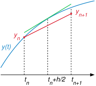
In numerical analysis, a branch of applied mathematics, the midpoint method is a one-step method for numerically solving the differential equation,
In mathematics, a stiff equation is a differential equation for which certain numerical methods for solving the equation are numerically unstable, unless the step size is taken to be extremely small. It has proven difficult to formulate a precise definition of stiffness, but the main idea is that the equation includes some terms that can lead to rapid variation in the solution.

In mathematics and computational science, the Euler method is a first-order numerical procedure for solving ordinary differential equations (ODEs) with a given initial value. It is the most basic explicit method for numerical integration of ordinary differential equations and is the simplest Runge–Kutta method. The Euler method is named after Leonhard Euler, who first proposed it in his book Institutionum calculi integralis.
In numerical analysis, finite-difference methods (FDM) are a class of numerical techniques for solving differential equations by approximating derivatives with finite differences. Both the spatial domain and time domain are discretized, or broken into a finite number of intervals, and the values of the solution at the end points of the intervals are approximated by solving algebraic equations containing finite differences and values from nearby points.
In mathematics of stochastic systems, the Runge–Kutta method is a technique for the approximate numerical solution of a stochastic differential equation. It is a generalisation of the Runge–Kutta method for ordinary differential equations to stochastic differential equations (SDEs). Importantly, the method does not involve knowing derivatives of the coefficient functions in the SDEs.
In mathematics, the Runge–Kutta–Fehlberg method is an algorithm in numerical analysis for the numerical solution of ordinary differential equations. It was developed by the German mathematician Erwin Fehlberg and is based on the large class of Runge–Kutta methods.
In mathematics and numerical analysis, an adaptive step size is used in some methods for the numerical solution of ordinary differential equations in order to control the errors of the method and to ensure stability properties such as A-stability. Using an adaptive stepsize is of particular importance when there is a large variation in the size of the derivative. For example, when modeling the motion of a satellite about the earth as a standard Kepler orbit, a fixed time-stepping method such as the Euler method may be sufficient. However things are more difficult if one wishes to model the motion of a spacecraft taking into account both the Earth and the Moon as in the Three-body problem. There, scenarios emerge where one can take large time steps when the spacecraft is far from the Earth and Moon, but if the spacecraft gets close to colliding with one of the planetary bodies, then small time steps are needed. Romberg's method and Runge–Kutta–Fehlberg are examples of a numerical integration methods which use an adaptive stepsize.
In numerical analysis, the Dormand–Prince (RKDP) method or DOPRI method, is an embedded method for solving ordinary differential equations (ODE). The method is a member of the Runge–Kutta family of ODE solvers. More specifically, it uses six function evaluations to calculate fourth- and fifth-order accurate solutions. The difference between these solutions is then taken to be the error of the (fourth-order) solution. This error estimate is very convenient for adaptive stepsize integration algorithms. Other similar integration methods are Fehlberg (RKF) and Cash–Karp (RKCK).
In mathematics and computational science, Heun's method may refer to the improved or modified Euler's method, or a similar two-stage Runge–Kutta method. It is named after Karl Heun and is a numerical procedure for solving ordinary differential equations (ODEs) with a given initial value. Both variants can be seen as extensions of the Euler method into two-stage second-order Runge–Kutta methods.
The Bogacki–Shampine method is a method for the numerical solution of ordinary differential equations, that was proposed by Przemysław Bogacki and Lawrence F. Shampine in 1989. The Bogacki–Shampine method is a Runge–Kutta method of order three with four stages with the First Same As Last (FSAL) property, so that it uses approximately three function evaluations per step. It has an embedded second-order method which can be used to implement adaptive step size. The Bogacki–Shampine method is implemented in the ode3 for fixed step solver and ode23 for a variable step solver function in MATLAB.
In numerical analysis, the Bulirsch–Stoer algorithm is a method for the numerical solution of ordinary differential equations which combines three powerful ideas: Richardson extrapolation, the use of rational function extrapolation in Richardson-type applications, and the modified midpoint method, to obtain numerical solutions to ordinary differential equations (ODEs) with high accuracy and comparatively little computational effort. It is named after Roland Bulirsch and Josef Stoer. It is sometimes called the Gragg–Bulirsch–Stoer (GBS) algorithm because of the importance of a result about the error function of the modified midpoint method, due to William B. Gragg.
In numerical analysis and scientific computing, the trapezoidal rule is a numerical method to solve ordinary differential equations derived from the trapezoidal rule for computing integrals. The trapezoidal rule is an implicit second-order method, which can be considered as both a Runge–Kutta method and a linear multistep method.
In numerical analysis and scientific computing, the Gauss–Legendre methods are a family of numerical methods for ordinary differential equations. Gauss–Legendre methods are implicit Runge–Kutta methods. More specifically, they are collocation methods based on the points of Gauss–Legendre quadrature. The Gauss–Legendre method based on s points has order 2s.
Exponential integrators are a class of numerical methods for the solution of ordinary differential equations, specifically initial value problems. This large class of methods from numerical analysis is based on the exact integration of the linear part of the initial value problem. Because the linear part is integrated exactly, this can help to mitigate the stiffness of a differential equation. Exponential integrators can be constructed to be explicit or implicit for numerical ordinary differential equations or serve as the time integrator for numerical partial differential equations.
The Segregated Runge–Kutta (SRK) method is a family of IMplicit–EXplicit (IMEX) Runge–Kutta methods that were developed to approximate the solution of differential algebraic equations (DAE) of index 2.
References
- J. R. Cash, A. H. Karp. "A variable order Runge-Kutta method for initial value problems with rapidly varying right-hand sides", ACM Transactions on Mathematical Software16: 201-222, 1990. doi : 10.1145/79505.79507.