Control-Lyapunov function

Last updated May 31, 2024

In control theory, a control-Lyapunov function (CLF)^[1]^[2]^[3]^[4] is an extension of the idea of Lyapunov function $V(x)$ to systems with control inputs. The ordinary Lyapunov function is used to test whether a dynamical system is (Lyapunov) stable or (more restrictively) asymptotically stable. Lyapunov stability means that if the system starts in a state $x\neq 0$ in some domain D, then the state will remain in D for all time. For asymptotic stability, the state is also required to converge to $x=0$ . A control-Lyapunov function is used to test whether a system is asymptotically stabilizable, that is whether for any state x there exists a control $u(x,t)$ such that the system can be brought to the zero state asymptotically by applying the control u.

Definition

Consider an autonomous dynamical system with inputs

{\dot {x}}=f(x,u)

(1)

where $x\in \mathbb {R} ^{n}$ is the state vector and $u\in \mathbb {R} ^{m}$ is the control vector. Suppose our goal is to drive the system to an equilibrium $x_{*}\in \mathbb {R} ^{n}$ from every initial state in some domain $D\subset \mathbb {R} ^{n}$ . Without loss of generality, suppose the equilibrium is at $x_{*}=0$ (for an equilibrium $x_{*}\neq 0$ , it can be translated to the origin by a change of variables).

Definition. A control-Lyapunov function (CLF) is a function $V:D\to \mathbb {R}$ that is continuously differentiable, positive-definite (that is, $V(x)$ is positive for all $x\in D$ except at $x=0$ where it is zero), and such that for all $x\in \mathbb {R} ^{n}(x\neq 0),$ there exists $u\in \mathbb {R} ^{m}$ such that

{\dot {V}}(x,u):=\langle \nabla V(x),f(x,u)\rangle <0,

where $\langle u,v\rangle$ denotes the inner product of $u,v\in \mathbb {R} ^{n}$ .

The last condition is the key condition; in words it says that for each state x we can find a control u that will reduce the "energy" V. Intuitively, if in each state we can always find a way to reduce the energy, we should eventually be able to bring the energy asymptotically to zero, that is to bring the system to a stop. This is made rigorous by Artstein's theorem.

Some results apply only to control-affine systems—i.e., control systems in the following form:

{\dot {x}}=f(x)+\sum _{i=1}^{m}g_{i}(x)u_{i}

(2)

where $f:\mathbb {R} ^{n}\to \mathbb {R} ^{n}$ and $g_{i}:\mathbb {R} ^{n}\to \mathbb {R} ^{n}$ for $i=1,\dots ,m$ .

Theorems

Eduardo Sontag showed that for a given control system, there exists a continuous CLF if and only if the origin is asymptotic stabilizable.^[5] It was later shown by Francis H. Clarke, Yuri Ledyaev, Eduardo Sontag, and A.I. Subbotin that every asymptotically controllable system can be stabilized by a (generally discontinuous) feedback.^[6] Artstein proved that the dynamical system ( 2 ) has a differentiable control-Lyapunov function if and only if there exists a regular stabilizing feedback u(x).

Constructing the Stabilizing Input

It is often difficult to find a control-Lyapunov function for a given system, but if one is found, then the feedback stabilization problem simplifies considerably. For the control affine system ( 2 ), Sontag's formula (or Sontag's universal formula) gives the feedback law $k:\mathbb {R} ^{n}\to \mathbb {R} ^{m}$ directly in terms of the derivatives of the CLF.^[4]^{: Eq. 5.56} In the special case of a single input system $(m=1)$ , Sontag's formula is written as

k(x)={\begin{cases}\displaystyle -{\frac {L_{f}V(x)+{\sqrt {\left[L_{f}V(x)\right]^{2}+\left[L_{g}V(x)\right]^{4}}}}{L_{g}V(x)}}&{\text{ if }}L_{g}V(x)\neq 0\\0&{\text{ if }}L_{g}V(x)=0\end{cases}}

where $L_{f}V(x):=\langle \nabla V(x),f(x)\rangle$ and $L_{g}V(x):=\langle \nabla V(x),g(x)\rangle$ are the Lie derivatives of $V$ along $f$ and $g$ , respectively.

For the general nonlinear system ( 1 ), the input $u$ can be found by solving a static non-linear programming problem

u^{*}(x)={\underset {u}{\operatorname {arg\,min} }}\nabla V(x)\cdot f(x,u)

for each state x.

Example

Here is a characteristic example of applying a Lyapunov candidate function to a control problem.

Consider the non-linear system, which is a mass-spring-damper system with spring hardening and position dependent mass described by

m(1+q^{2}){\ddot {q}}+b{\dot {q}}+K_{0}q+K_{1}q^{3}=u

Now given the desired state, $q_{d}$ , and actual state, $q$ , with error, $e=q_{d}-q$ , define a function $r$ as

r={\dot {e}}+\alpha e

A Control-Lyapunov candidate is then

r\mapsto V(r):={\frac {1}{2}}r^{2}

which is positive for all $r\neq 0$ .

Now taking the time derivative of $V$

{\dot {V}}=r{\dot {r}}

{\dot {V}}=({\dot {e}}+\alpha e)({\ddot {e}}+\alpha {\dot {e}})

The goal is to get the time derivative to be

{\dot {V}}=-\kappa V

which is globally exponentially stable if $V$ is globally positive definite (which it is).

Hence we want the rightmost bracket of ${\dot {V}}$ ,

({\ddot {e}}+\alpha {\dot {e}})=({\ddot {q}}_{d}-{\ddot {q}}+\alpha {\dot {e}})

to fulfill the requirement

({\ddot {q}}_{d}-{\ddot {q}}+\alpha {\dot {e}})=-{\frac {\kappa }{2}}({\dot {e}}+\alpha e)

which upon substitution of the dynamics, ${\ddot {q}}$ , gives

\left({\ddot {q}}_{d}-{\frac {u-K_{0}q-K_{1}q^{3}-b{\dot {q}}}{m(1+q^{2})}}+\alpha {\dot {e}}\right)=-{\frac {\kappa }{2}}({\dot {e}}+\alpha e)

Solving for $u$ yields the control law

u=m(1+q^{2})\left({\ddot {q}}_{d}+\alpha {\dot {e}}+{\frac {\kappa }{2}}r\right)+K_{0}q+K_{1}q^{3}+b{\dot {q}}

with $\kappa$ and $\alpha$ , both greater than zero, as tunable parameters

This control law will guarantee global exponential stability since upon substitution into the time derivative yields, as expected

{\dot {V}}=-\kappa V

which is a linear first order differential equation which has solution

V=V(0)\exp(-\kappa t)

And hence the error and error rate, remembering that $V={\frac {1}{2}}({\dot {e}}+\alpha e)^{2}$ , exponentially decay to zero.

If you wish to tune a particular response from this, it is necessary to substitute back into the solution we derived for $V$ and solve for $e$ . This is left as an exercise for the reader but the first few steps at the solution are:

r{\dot {r}}=-{\frac {\kappa }{2}}r^{2}

{\dot {r}}=-{\frac {\kappa }{2}}r

r=r(0)\exp \left(-{\frac {\kappa }{2}}t\right)

{\dot {e}}+\alpha e=({\dot {e}}(0)+\alpha e(0))\exp \left(-{\frac {\kappa }{2}}t\right)

which can then be solved using any linear differential equation methods.

Related Research Articles

Continuum mechanics is a branch of mechanics that deals with the deformation of and transmission of forces through materials modeled as a continuous medium rather than as discrete particles. The French mathematician Augustin-Louis Cauchy was the first to formulate such models in the 19th century.

In mathematics, particularly linear algebra and numerical analysis, the Gram–Schmidt process or Gram-Schmidt algorithm is a way of finding a set of two or more vectors that are perpendicular to each other.

In the theory of ordinary differential equations (ODEs), Lyapunov functions, named after Aleksandr Lyapunov, are scalar functions that may be used to prove the stability of an equilibrium of an ODE. Lyapunov functions are important to stability theory of dynamical systems and control theory. A similar concept appears in the theory of general state-space Markov chains usually under the name Foster–Lyapunov functions.

Various types of stability may be discussed for the solutions of differential equations or difference equations describing dynamical systems. The most important type is that concerning the stability of solutions near to a point of equilibrium. This may be discussed by the theory of Aleksandr Lyapunov. In simple terms, if the solutions that start out near an equilibrium point $stay near forever, then is Lyapunov stable . More strongly, if is Lyapunov stable and all solutions that start out near converge to, then is said to be asymptotically stable . The notion of exponential stability guarantees a minimal rate of decay, i.e., an estimate of how quickly the solutions converge. The idea of Lyapunov stability can be extended to infinite-dimensional manifolds, where it is known as structural stability, which concerns the behavior of different but "nearby" solutions to differential equations. Input-to-state stability (ISS) applies Lyapunov notions to systems with inputs.$

In control systems, sliding mode control (SMC) is a nonlinear control method that alters the dynamics of a nonlinear system by applying a discontinuous control signal that forces the system to "slide" along a cross-section of the system's normal behavior. The state-feedback control law is not a continuous function of time. Instead, it can switch from one continuous structure to another based on the current position in the state space. Hence, sliding mode control is a variable structure control method. The multiple control structures are designed so that trajectories always move toward an adjacent region with a different control structure, and so the ultimate trajectory will not exist entirely within one control structure. Instead, it will slide along the boundaries of the control structures. The motion of the system as it slides along these boundaries is called a sliding mode and the geometrical locus consisting of the boundaries is called the sliding (hyper)surface. In the context of modern control theory, any variable structure system, like a system under SMC, may be viewed as a special case of a hybrid dynamical system as the system both flows through a continuous state space but also moves through different discrete control modes.

In physics, the S-matrix or scattering matrix relates the initial state and the final state of a physical system undergoing a scattering process. It is used in quantum mechanics, scattering theory and quantum field theory (QFT).

<span class="mw-page-title-main">Envelope (mathematics)</span> Curve external to a family of curves in geometry

In geometry, an envelope of a planar family of curves is a curve that is tangent to each member of the family at some point, and these points of tangency together form the whole envelope. Classically, a point on the envelope can be thought of as the intersection of two "infinitesimally adjacent" curves, meaning the limit of intersections of nearby curves. This idea can be generalized to an envelope of surfaces in space, and so on to higher dimensions.

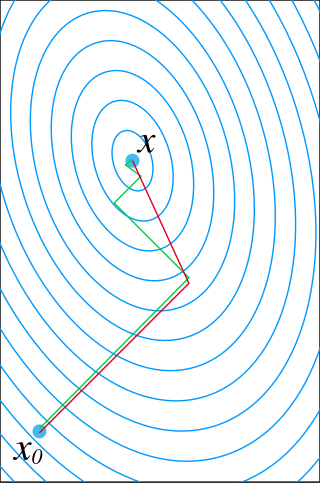
In mathematics, the conjugate gradient method is an algorithm for the numerical solution of particular systems of linear equations, namely those whose matrix is positive-semidefinite. The conjugate gradient method is often implemented as an iterative algorithm, applicable to sparse systems that are too large to be handled by a direct implementation or other direct methods such as the Cholesky decomposition. Large sparse systems often arise when numerically solving partial differential equations or optimization problems.

In differential geometry, a tensor density or relative tensor is a generalization of the tensor field concept. A tensor density transforms as a tensor field when passing from one coordinate system to another, except that it is additionally multiplied or weighted by a power W of the Jacobian determinant of the coordinate transition function or its absolute value. A tensor density with a single index is called a vector density. A distinction is made among (authentic) tensor densities, pseudotensor densities, even tensor densities and odd tensor densities. Sometimes tensor densities with a negative weight W are called tensor capacity. A tensor density can also be regarded as a section of the tensor product of a tensor bundle with a density bundle.

An osculating circle is a circle that best approximates the curvature of a curve at a specific point. It is tangent to the curve at that point and has the same curvature as the curve at that point. The osculating circle provides a way to understand the local behavior of a curve and is commonly used in differential geometry and calculus.

In applied mathematics, comparison functions are several classes of continuous functions, which are used in stability theory to characterize the stability properties of control systems as Lyapunov stability, uniform asymptotic stability etc.

In directional statistics, the von Mises–Fisher distribution, is a probability distribution on the $-sphere in . If the distribution reduces to the von Mises distribution on the circle.$

The Newman–Penrose (NP) formalism is a set of notation developed by Ezra T. Newman and Roger Penrose for general relativity (GR). Their notation is an effort to treat general relativity in terms of spinor notation, which introduces complex forms of the usual variables used in GR. The NP formalism is itself a special case of the tetrad formalism, where the tensors of the theory are projected onto a complete vector basis at each point in spacetime. Usually this vector basis is chosen to reflect some symmetry of the spacetime, leading to simplified expressions for physical observables. In the case of the NP formalism, the vector basis chosen is a null tetrad: a set of four null vectors—two real, and a complex-conjugate pair. The two real members often asymptotically point radially inward and radially outward, and the formalism is well adapted to treatment of the propagation of radiation in curved spacetime. The Weyl scalars, derived from the Weyl tensor, are often used. In particular, it can be shown that one of these scalars— $in the appropriate frame—encodes the outgoing gravitational radiation of an asymptotically flat system.$

In celestial mechanics, a Kepler orbit is the motion of one body relative to another, as an ellipse, parabola, or hyperbola, which forms a two-dimensional orbital plane in three-dimensional space. A Kepler orbit can also form a straight line. It considers only the point-like gravitational attraction of two bodies, neglecting perturbations due to gravitational interactions with other objects, atmospheric drag, solar radiation pressure, a non-spherical central body, and so on. It is thus said to be a solution of a special case of the two-body problem, known as the Kepler problem. As a theory in classical mechanics, it also does not take into account the effects of general relativity. Keplerian orbits can be parametrized into six orbital elements in various ways.

Anatoly Alexeyevich Karatsuba was a Russian mathematician working in the field of analytic number theory, p-adic numbers and Dirichlet series.

<span class="mw-page-title-main">Plate theory</span> Mathematical model of the stresses within flat plates under loading

In continuum mechanics, plate theories are mathematical descriptions of the mechanics of flat plates that draw on the theory of beams. Plates are defined as plane structural elements with a small thickness compared to the planar dimensions. The typical thickness to width ratio of a plate structure is less than 0.1. A plate theory takes advantage of this disparity in length scale to reduce the full three-dimensional solid mechanics problem to a two-dimensional problem. The aim of plate theory is to calculate the deformation and stresses in a plate subjected to loads.

The Reissner–Mindlin theory of plates is an extension of Kirchhoff–Love plate theory that takes into account shear deformations through-the-thickness of a plate. The theory was proposed in 1951 by Raymond Mindlin. A similar, but not identical, theory in static setting, had been proposed earlier by Eric Reissner in 1945. Both theories are intended for thick plates in which the normal to the mid-surface remains straight but not necessarily perpendicular to the mid-surface. The Reissner-Mindlin theory is used to calculate the deformations and stresses in a plate whose thickness is of the order of one tenth the planar dimensions while the Kirchhoff–Love theory is applicable to thinner plates.

Heat transfer physics describes the kinetics of energy storage, transport, and energy transformation by principal energy carriers: phonons, electrons, fluid particles, and photons. Heat is thermal energy stored in temperature-dependent motion of particles including electrons, atomic nuclei, individual atoms, and molecules. Heat is transferred to and from matter by the principal energy carriers. The state of energy stored within matter, or transported by the carriers, is described by a combination of classical and quantum statistical mechanics. The energy is different made (converted) among various carriers. The heat transfer processes are governed by the rates at which various related physical phenomena occur, such as the rate of particle collisions in classical mechanics. These various states and kinetics determine the heat transfer, i.e., the net rate of energy storage or transport. Governing these process from the atomic level to macroscale are the laws of thermodynamics, including conservation of energy.

Input-to-state stability (ISS) is a stability notion widely used to study stability of nonlinear control systems with external inputs. Roughly speaking, a control system is ISS if it is globally asymptotically stable in the absence of external inputs and if its trajectories are bounded by a function of the size of the input for all sufficiently large times. The importance of ISS is due to the fact that the concept has bridged the gap between input–output and state-space methods, widely used within the control systems community.

The Kaniadakis Weibull distribution is a probability distribution arising as a generalization of the Weibull distribution. It is one example of a Kaniadakis κ-distribution. The κ-Weibull distribution has been adopted successfully for describing a wide variety of complex systems in seismology, economy, epidemiology, among many others.

References

↑ Isidori, A. (1995). Nonlinear Control Systems. Springer. ISBN 978-3-540-19916-8.
↑ Freeman, Randy A.; Petar V. Kokotović (2008). "Robust Control Lyapunov Functions". Robust Nonlinear Control Design (illustrated, reprint ed.). Birkhäuser. pp. 33–63. doi:10.1007/978-0-8176-4759-9_3. ISBN 978-0-8176-4758-2 . Retrieved 2009-03-04.
↑ Khalil, Hassan (2015). Nonlinear Control. Pearson. ISBN 9780133499261.
1 2 Sontag, Eduardo (1998). Mathematical Control Theory: Deterministic Finite Dimensional Systems. Second Edition (PDF). Springer. ISBN 978-0-387-98489-6.
↑ Sontag, E.D. (1983). "A Lyapunov-like characterization of asymptotic controllability". SIAM J. Control Optim. 21 (3): 462–471. doi:10.1137/0321028. S2CID 450209.
↑ Clarke, F.H.; Ledyaev, Y.S.; Sontag, E.D.; Subbotin, A.I. (1997). "Asymptotic controllability implies feedback stabilization". IEEE Trans. Autom. Control. 42 (10): 1394–1407. doi:10.1109/9.633828.