Dynamical system

This article is about the general aspects of dynamical systems. For the study field, see Dynamical systems theory.

"Dynamical" redirects here. For other uses, see Dynamical (disambiguation).

The Lorenz attractor arises in the study of the Lorenz oscillator, a dynamical system.

In mathematics, a dynamical system is a system in which a function describes the time dependence of a point in an ambient space, such as in a parametric curve. Examples include the mathematical models that describe the swinging of a clock pendulum, the flow of water in a pipe, the random motion of particles in the air, and the number of fish each springtime in a lake. The most general definition unifies several concepts in mathematics such as ordinary differential equations and ergodic theory by allowing different choices of the space and how time is measured.^{[ citation needed ]} Time can be measured by integers, by real or complex numbers or can be a more general algebraic object, losing the memory of its physical origin, and the space may be a manifold or simply a set, without the need of a smooth space-time structure defined on it.

At any given time, a dynamical system has a state representing a point in an appropriate state space. This state is often given by a tuple of real numbers or by a vector in a geometrical manifold. The evolution rule of the dynamical system is a function that describes what future states follow from the current state. Often the function is deterministic, that is, for a given time interval only one future state follows from the current state. ^{[1] [2]} However, some systems are stochastic, in that random events also affect the evolution of the state variables.

In physics, a dynamical system is described as a "particle or ensemble of particles whose state varies over time and thus obeys differential equations involving time derivatives". ^[3] In order to make a prediction about the system's future behavior, an analytical solution of such equations or their integration over time through computer simulation is realized.

The study of dynamical systems is the focus of dynamical systems theory, which has applications to a wide variety of fields such as mathematics, physics, ^{[4] [5]} biology, ^[6] chemistry, engineering, ^[7] economics, ^[8] history, and medicine. Dynamical systems are a fundamental part of chaos theory, logistic map dynamics, bifurcation theory, the self-assembly and self-organization processes, and the edge of chaos concept.

Overview

The concept of a dynamical system has its origins in Newtonian mechanics. There, as in other natural sciences and engineering disciplines, the evolution rule of dynamical systems is an implicit relation that gives the state of the system for only a short time into the future. (The relation is either a differential equation, difference equation or other time scale.) To determine the state for all future times requires iterating the relation many times—each advancing time a small step. The iteration procedure is referred to as solving the system or integrating the system. If the system can be solved, then, given an initial point, it is possible to determine all its future positions, a collection of points known as a trajectory or orbit .

Before the advent of computers, finding an orbit required sophisticated mathematical techniques and could be accomplished only for a small class of dynamical systems. Numerical methods implemented on electronic computing machines have simplified the task of determining the orbits of a dynamical system.

For simple dynamical systems, knowing the trajectory is often sufficient, but most dynamical systems are too complicated to be understood in terms of individual trajectories. The difficulties arise because:

• The systems studied may only be known approximately—the parameters of the system may not be known precisely or terms may be missing from the equations. The approximations used bring into question the validity or relevance of numerical solutions. To address these questions several notions of stability have been introduced in the study of dynamical systems, such as Lyapunov stability or structural stability. The stability of the dynamical system implies that there is a class of models or initial conditions for which the trajectories would be equivalent. The operation for comparing orbits to establish their equivalence changes with the different notions of stability.
• The type of trajectory may be more important than one particular trajectory. Some trajectories may be periodic, whereas others may wander through many different states of the system. Applications often require enumerating these classes or maintaining the system within one class. Classifying all possible trajectories has led to the qualitative study of dynamical systems, that is, properties that do not change under coordinate changes. Linear dynamical systems and systems that have two numbers describing a state are examples of dynamical systems where the possible classes of orbits are understood.
• The behavior of trajectories as a function of a parameter may be what is needed for an application. As a parameter is varied, the dynamical systems may have bifurcation points where the qualitative behavior of the dynamical system changes. For example, it may go from having only periodic motions to apparently erratic behavior, as in the transition to turbulence of a fluid.
• The trajectories of the system may appear erratic, as if random. In these cases it may be necessary to compute averages using one very long trajectory or many different trajectories. The averages are well defined for ergodic systems and a more detailed understanding has been worked out for hyperbolic systems. Understanding the probabilistic aspects of dynamical systems has helped establish the foundations of statistical mechanics and of chaos.

History

Many people regard French mathematician Henri Poincaré as the founder of dynamical systems. ^[9] Poincaré published two now classical monographs, "New Methods of Celestial Mechanics" (1892–1899) and "Lectures on Celestial Mechanics" (1905–1910). In them, he successfully applied the results of their research to the problem of the motion of three bodies and studied in detail the behavior of solutions (frequency, stability, asymptotic, and so on). These papers included the Poincaré recurrence theorem, which states that certain systems will, after a sufficiently long but finite time, return to a state very close to the initial state.

Aleksandr Lyapunov developed many important approximation methods. His methods, which he developed in 1899, make it possible to define the stability of sets of ordinary differential equations. He created the modern theory of the stability of a dynamical system.

In 1913, George David Birkhoff proved Poincaré's "Last Geometric Theorem", a special case of the three-body problem, a result that made him world-famous. In 1927, he published his Dynamical Systems . Birkhoff's most durable result has been his 1931 discovery of what is now called the ergodic theorem. Combining insights from physics on the ergodic hypothesis with measure theory, this theorem solved, at least in principle, a fundamental problem of statistical mechanics. The ergodic theorem has also had repercussions for dynamics.

Stephen Smale made significant advances as well. His first contribution was the Smale horseshoe that jumpstarted significant research in dynamical systems. He also outlined a research program carried out by many others.

Oleksandr Mykolaiovych Sharkovsky developed Sharkovsky's theorem on the periods of discrete dynamical systems in 1964. One of the implications of the theorem is that if a discrete dynamical system on the real line has a periodic point of period 3, then it must have periodic points of every other period.

In the late 20th century the dynamical system perspective to partial differential equations started gaining popularity. Palestinian mechanical engineer Ali H. Nayfeh applied nonlinear dynamics in mechanical and engineering systems. ^[10] His pioneering work in applied nonlinear dynamics has been influential in the construction and maintenance of machines and structures that are common in daily life, such as ships, cranes, bridges, buildings, skyscrapers, jet engines, rocket engines, aircraft and spacecraft. ^[11]

Formal definition

In the most general sense, ^{[12] [13]} a dynamical system is a tuple (T, X, Φ) where T is a monoid, written additively, X is a non-empty set and Φ is a function

${\displaystyle \Phi :U\subseteq (T\times X)\to X}$

with

${\displaystyle \mathrm {proj} _{2}(U)=X}$ (where ${\displaystyle \mathrm {proj} _{2}}$ is the 2nd projection map)

and for any x in X:

${\displaystyle \Phi (0,x)=x}$

${\displaystyle \Phi (t_{2},\Phi (t_{1},x))=\Phi (t_{2}+t_{1},x),}$

for ${\displaystyle \,t_{1},\,t_{2}+t_{1}\in I(x)}$ and ${\displaystyle \ t_{2}\in I(\Phi (t_{1},x))}$, where we have defined the set ${\displaystyle I(x):=\{t\in T:(t,x)\in U\}}$ for any x in X.

In particular, in the case that ${\displaystyle U=T\times X}$ we have for every x in X that ${\displaystyle I(x)=T}$ and thus that Φ defines a monoid action of T on X.

The function Φ(t,x) is called the evolution function of the dynamical system: it associates to every point x in the set X a unique image, depending on the variable t, called the evolution parameter. X is called phase space or state space, while the variable x represents an initial state of the system.

We often write

${\displaystyle \Phi _{x}(t)\equiv \Phi (t,x)}$

${\displaystyle \Phi ^{t}(x)\equiv \Phi (t,x)}$

if we take one of the variables as constant. The function

${\displaystyle \Phi _{x}:I(x)\to X}$

is called the flow through x and its graph is called the trajectory through x. The set

${\displaystyle \gamma _{x}\equiv \{\Phi (t,x):t\in I(x)\}}$

is called the orbit through x. The orbit through x is the image of the flow through x. A subset S of the state space X is called Φ-invariant if for all x in S and all t in T

${\displaystyle \Phi (t,x)\in S.}$

Thus, in particular, if S is Φ-invariant,${\displaystyle I(x)=T}$ for all x in S. That is, the flow through x must be defined for all time for every element of S.

More commonly there are two classes of definitions for a dynamical system: one is motivated by ordinary differential equations and is geometrical in flavor; and the other is motivated by ergodic theory and is measure theoretical in flavor.

Geometrical definition

In the geometrical definition, a dynamical system is the tuple ${\displaystyle \langle {\mathcal {T}},{\mathcal {M}},f\rangle }$. ${\displaystyle {\mathcal {T}}}$ is the domain for time – there are many choices, usually the reals or the integers, possibly restricted to be non-negative. ${\displaystyle {\mathcal {M}}}$ is a manifold, i.e. locally a Banach space or Euclidean space, or in the discrete case a graph. f is an evolution rule t → f ^t (with ${\displaystyle t\in {\mathcal {T}}}$) such that f ^t is a diffeomorphism of the manifold to itself. So, f is a "smooth" mapping of the time-domain ${\displaystyle {\mathcal {T}}}$ into the space of diffeomorphisms of the manifold to itself. In other terms, f(t) is a diffeomorphism, for every time t in the domain ${\displaystyle {\mathcal {T}}}$ .

Real dynamical system

A real dynamical system, real-time dynamical system, continuous time dynamical system, or flow is a tuple (T, M, Φ) with T an open interval in the real numbers R, M a manifold locally diffeomorphic to a Banach space, and Φ a continuous function. If Φ is continuously differentiable we say the system is a differentiable dynamical system. If the manifold M is locally diffeomorphic to Rⁿ, the dynamical system is finite-dimensional; if not, the dynamical system is infinite-dimensional. This does not assume a symplectic structure. When T is taken to be the reals, the dynamical system is called global or a flow ; and if T is restricted to the non-negative reals, then the dynamical system is a semi-flow.

Discrete dynamical system

A discrete dynamical system, discrete-time dynamical system is a tuple (T, M, Φ), where M is a manifold locally diffeomorphic to a Banach space, and Φ is a function. When T is taken to be the integers, it is a cascade or a map. If T is restricted to the non-negative integers we call the system a semi-cascade. ^[14]

Cellular automaton

A cellular automaton is a tuple (T, M, Φ), with T a lattice such as the integers or a higher-dimensional integer grid, M is a set of functions from an integer lattice (again, with one or more dimensions) to a finite set, and Φ a (locally defined) evolution function. As such cellular automata are dynamical systems. The lattice in M represents the "space" lattice, while the one in T represents the "time" lattice.

Multidimensional generalization

Dynamical systems are usually defined over a single independent variable, thought of as time. A more general class of systems are defined over multiple independent variables and are therefore called multidimensional systems. Such systems are useful for modeling, for example, image processing.

Compactification of a dynamical system

Given a global dynamical system (R, X, Φ) on a locally compact and Hausdorff topological space X, it is often useful to study the continuous extension Φ* of Φ to the one-point compactification X* of X. Although we lose the differential structure of the original system we can now use compactness arguments to analyze the new system (R, X*, Φ*).

In compact dynamical systems the limit set of any orbit is non-empty, compact and simply connected.

Measure theoretical definition

Main article: Measure-preserving dynamical system

A dynamical system may be defined formally as a measure-preserving transformation of a measure space, the triplet (T, (X, Σ, μ), Φ). Here, T is a monoid (usually the non-negative integers), X is a set, and (X, Σ, μ) is a probability space, meaning that Σ is a sigma-algebra on X and μ is a finite measure on (X, Σ). A map Φ: X → X is said to be Σ-measurable if and only if, for every σ in Σ, one has ${\displaystyle \Phi ^{-1}\sigma \in \Sigma }$. A map Φ is said to preserve the measure if and only if, for every σ in Σ, one has ${\displaystyle \mu (\Phi ^{-1}\sigma )=\mu (\sigma )}$. Combining the above, a map Φ is said to be a measure-preserving transformation of X, if it is a map from X to itself, it is Σ-measurable, and is measure-preserving. The triplet (T, (X, Σ, μ), Φ), for such a Φ, is then defined to be a dynamical system.

The map Φ embodies the time evolution of the dynamical system. Thus, for discrete dynamical systems the iterates ${\displaystyle \Phi ^{n}=\Phi \circ \Phi \circ \dots \circ \Phi }$ for every integer n are studied. For continuous dynamical systems, the map Φ is understood to be a finite time evolution map and the construction is more complicated.

Relation to geometric definition

The measure theoretical definition assumes the existence of a measure-preserving transformation. Many different invariant measures can be associated to any one evolution rule. If the dynamical system is given by a system of differential equations the appropriate measure must be determined. This makes it difficult to develop ergodic theory starting from differential equations, so it becomes convenient to have a dynamical systems-motivated definition within ergodic theory that side-steps the choice of measure and assumes the choice has been made. A simple construction (sometimes called the Krylov–Bogolyubov theorem) shows that for a large class of systems it is always possible to construct a measure so as to make the evolution rule of the dynamical system a measure-preserving transformation. In the construction a given measure of the state space is summed for all future points of a trajectory, assuring the invariance.

Some systems have a natural measure, such as the Liouville measure in Hamiltonian systems, chosen over other invariant measures, such as the measures supported on periodic orbits of the Hamiltonian system. For chaotic dissipative systems the choice of invariant measure is technically more challenging. The measure needs to be supported on the attractor, but attractors have zero Lebesgue measure and the invariant measures must be singular with respect to the Lebesgue measure. A small region of phase space shrinks under time evolution.

For hyperbolic dynamical systems, the Sinai–Ruelle–Bowen measures appear to be the natural choice. They are constructed on the geometrical structure of stable and unstable manifolds of the dynamical system; they behave physically under small perturbations; and they explain many of the observed statistics of hyperbolic systems.

Construction of dynamical systems

The concept of evolution in time is central to the theory of dynamical systems as seen in the previous sections: the basic reason for this fact is that the starting motivation of the theory was the study of time behavior of classical mechanical systems. But a system of ordinary differential equations must be solved before it becomes a dynamic system. For example consider an initial value problem such as the following:

${\displaystyle {\dot {\boldsymbol {x}}}={\boldsymbol {v}}(t,{\boldsymbol {x}})}$

${\displaystyle {\boldsymbol {x}}|_{t=0}={\boldsymbol {x}}_{0}}$

where

• ${\displaystyle {\dot {\boldsymbol {x}}}}$ represents the velocity of the material point x
• M is a finite dimensional manifold
• v: T × M → TM is a vector field in Rⁿ or Cⁿ and represents the change of velocity induced by the known forces acting on the given material point in the phase space M. The change is not a vector in the phase space M, but is instead in the tangent space TM.

There is no need for higher order derivatives in the equation, nor for the parameter t in v(t,x), because these can be eliminated by considering systems of higher dimensions.

Depending on the properties of this vector field, the mechanical system is called

• autonomous, when v(t, x) = v(x)
• homogeneous when v(t, 0) = 0 for all t

The solution can be found using standard ODE techniques and is denoted as the evolution function already introduced above

${\displaystyle {\boldsymbol {x}}(t)=\Phi (t,{\boldsymbol {x}}_{0})}$

The dynamical system is then (T, M, Φ).

Some formal manipulation of the system of differential equations shown above gives a more general form of equations a dynamical system must satisfy

${\displaystyle {\dot {\boldsymbol {x}}}-{\boldsymbol {v}}(t,{\boldsymbol {x}})=0\qquad \Leftrightarrow \qquad {\mathfrak {G}}\left(t,\Phi (t,{\boldsymbol {x}}_{0})\right)=0}$

where ${\displaystyle {\mathfrak {G}}:{{(T\times M)}^{M}}\to \mathbf {C} }$ is a functional from the set of evolution functions to the field of the complex numbers.

This equation is useful when modeling mechanical systems with complicated constraints.

Many of the concepts in dynamical systems can be extended to infinite-dimensional manifolds—those that are locally Banach spaces—in which case the differential equations are partial differential equations.

Examples

• Arnold's cat map
• Baker's map is an example of a chaotic piecewise linear map
• Billiards and outer billiards
• Bouncing ball dynamics
• Circle map
• Complex quadratic polynomial
• Double pendulum
• Dyadic transformation
• Hénon map
• Irrational rotation
• Kaplan–Yorke map
• List of chaotic maps
• Lorenz system
• Quadratic map simulation system
• Rössler map
• Swinging Atwood's machine
• Tent map

Linear dynamical systems

Main article: Linear dynamical system

Linear dynamical systems can be solved in terms of simple functions and the behavior of all orbits classified. In a linear system the phase space is the N-dimensional Euclidean space, so any point in phase space can be represented by a vector with N numbers. The analysis of linear systems is possible because they satisfy a superposition principle: if u(t) and w(t) satisfy the differential equation for the vector field (but not necessarily the initial condition), then so will u(t) + w(t).

Flows

For a flow, the vector field v(x) is an affine function of the position in the phase space, that is,

${\displaystyle {\dot {x}}=v(x)=Ax+b,}$

with A a matrix, b a vector of numbers and x the position vector. The solution to this system can be found by using the superposition principle (linearity). The case b ≠ 0 with A = 0 is just a straight line in the direction of b:

${\displaystyle \Phi ^{t}(x_{1})=x_{1}+bt.}$

When b is zero and A ≠ 0 the origin is an equilibrium (or singular) point of the flow, that is, if x₀ = 0, then the orbit remains there. For other initial conditions, the equation of motion is given by the exponential of a matrix: for an initial point x₀,

${\displaystyle \Phi ^{t}(x_{0})=e^{tA}x_{0}.}$

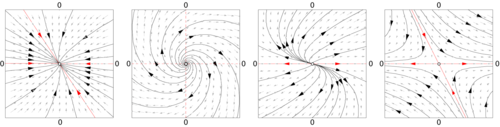
When b = 0, the eigenvalues of A determine the structure of the phase space. From the eigenvalues and the eigenvectors of A it is possible to determine if an initial point will converge or diverge to the equilibrium point at the origin.

The distance between two different initial conditions in the case A ≠ 0 will change exponentially in most cases, either converging exponentially fast towards a point, or diverging exponentially fast. Linear systems display sensitive dependence on initial conditions in the case of divergence. For nonlinear systems this is one of the (necessary but not sufficient) conditions for chaotic behavior.

Linear vector fields and a few trajectories.

Maps

A discrete-time, affine dynamical system has the form of a matrix difference equation:

${\displaystyle x_{n+1}=Ax_{n}+b,}$

with A a matrix and b a vector. As in the continuous case, the change of coordinates x → x + (1 − A) ^–1b removes the term b from the equation. In the new coordinate system, the origin is a fixed point of the map and the solutions are of the linear system A ⁿx₀. The solutions for the map are no longer curves, but points that hop in the phase space. The orbits are organized in curves, or fibers, which are collections of points that map into themselves under the action of the map.

As in the continuous case, the eigenvalues and eigenvectors of A determine the structure of phase space. For example, if u₁ is an eigenvector of A, with a real eigenvalue smaller than one, then the straight lines given by the points along α u₁, with α ∈ R, is an invariant curve of the map. Points in this straight line run into the fixed point.

There are also many other discrete dynamical systems.

Local dynamics

The qualitative properties of dynamical systems do not change under a smooth change of coordinates (this is sometimes taken as a definition of qualitative): a singular point of the vector field (a point where v(x) = 0) will remain a singular point under smooth transformations; a periodic orbit is a loop in phase space and smooth deformations of the phase space cannot alter it being a loop. It is in the neighborhood of singular points and periodic orbits that the structure of a phase space of a dynamical system can be well understood. In the qualitative study of dynamical systems, the approach is to show that there is a change of coordinates (usually unspecified, but computable) that makes the dynamical system as simple as possible.

Rectification

A flow in most small patches of the phase space can be made very simple. If y is a point where the vector field v(y) ≠ 0, then there is a change of coordinates for a region around y where the vector field becomes a series of parallel vectors of the same magnitude. This is known as the rectification theorem.

The rectification theorem says that away from singular points the dynamics of a point in a small patch is a straight line. The patch can sometimes be enlarged by stitching several patches together, and when this works out in the whole phase space M the dynamical system is integrable. In most cases the patch cannot be extended to the entire phase space. There may be singular points in the vector field (where v(x) = 0); or the patches may become smaller and smaller as some point is approached. The more subtle reason is a global constraint, where the trajectory starts out in a patch, and after visiting a series of other patches comes back to the original one. If the next time the orbit loops around phase space in a different way, then it is impossible to rectify the vector field in the whole series of patches.

Near periodic orbits

In general, in the neighborhood of a periodic orbit the rectification theorem cannot be used. Poincaré developed an approach that transforms the analysis near a periodic orbit to the analysis of a map. Pick a point x₀ in the orbit γ and consider the points in phase space in that neighborhood that are perpendicular to v(x₀). These points are a Poincaré section S(γ, x₀), of the orbit. The flow now defines a map, the Poincaré map F : S → S, for points starting in S and returning to S. Not all these points will take the same amount of time to come back, but the times will be close to the time it takes x₀.

The intersection of the periodic orbit with the Poincaré section is a fixed point of the Poincaré map F. By a translation, the point can be assumed to be at x = 0. The Taylor series of the map is F(x) = J · x + O(x²), so a change of coordinates h can only be expected to simplify F to its linear part

${\displaystyle h^{-1}\circ F\circ h(x)=J\cdot x.}$

This is known as the conjugation equation. Finding conditions for this equation to hold has been one of the major tasks of research in dynamical systems. Poincaré first approached it assuming all functions to be analytic and in the process discovered the non-resonant condition. If λ₁, ..., λ_ν are the eigenvalues of J they will be resonant if one eigenvalue is an integer linear combination of two or more of the others. As terms of the form λ_i – Σ (multiples of other eigenvalues) occurs in the denominator of the terms for the function h, the non-resonant condition is also known as the small divisor problem.

Conjugation results

The results on the existence of a solution to the conjugation equation depend on the eigenvalues of J and the degree of smoothness required from h. As J does not need to have any special symmetries, its eigenvalues will typically be complex numbers. When the eigenvalues of J are not in the unit circle, the dynamics near the fixed point x₀ of F is called hyperbolic and when the eigenvalues are on the unit circle and complex, the dynamics is called elliptic.

In the hyperbolic case, the Hartman–Grobman theorem gives the conditions for the existence of a continuous function that maps the neighborhood of the fixed point of the map to the linear map J · x. The hyperbolic case is also structurally stable. Small changes in the vector field will only produce small changes in the Poincaré map and these small changes will reflect in small changes in the position of the eigenvalues of J in the complex plane, implying that the map is still hyperbolic.

The Kolmogorov–Arnold–Moser (KAM) theorem gives the behavior near an elliptic point.

Bifurcation theory

Main article: Bifurcation theory

When the evolution map Φ^t (or the vector field it is derived from) depends on a parameter μ, the structure of the phase space will also depend on this parameter. Small changes may produce no qualitative changes in the phase space until a special value μ₀ is reached. At this point the phase space changes qualitatively and the dynamical system is said to have gone through a bifurcation.

Bifurcation theory considers a structure in phase space (typically a fixed point, a periodic orbit, or an invariant torus) and studies its behavior as a function of the parameter μ. At the bifurcation point the structure may change its stability, split into new structures, or merge with other structures. By using Taylor series approximations of the maps and an understanding of the differences that may be eliminated by a change of coordinates, it is possible to catalog the bifurcations of dynamical systems.

The bifurcations of a hyperbolic fixed point x₀ of a system family F_μ can be characterized by the eigenvalues of the first derivative of the system DF_μ(x₀) computed at the bifurcation point. For a map, the bifurcation will occur when there are eigenvalues of DF_μ on the unit circle. For a flow, it will occur when there are eigenvalues on the imaginary axis. For more information, see the main article on Bifurcation theory.

Some bifurcations can lead to very complicated structures in phase space. For example, the Ruelle–Takens scenario describes how a periodic orbit bifurcates into a torus and the torus into a strange attractor. In another example, Feigenbaum period-doubling describes how a stable periodic orbit goes through a series of period-doubling bifurcations.

Ergodic systems

Main article: Ergodic theory

In many dynamical systems, it is possible to choose the coordinates of the system so that the volume (really a ν-dimensional volume) in phase space is invariant. This happens for mechanical systems derived from Newton's laws as long as the coordinates are the position and the momentum and the volume is measured in units of (position) × (momentum). The flow takes points of a subset A into the points Φ ^t(A) and invariance of the phase space means that

${\displaystyle \mathrm {vol} (A)=\mathrm {vol} (\Phi ^{t}(A)).}$

In the Hamiltonian formalism, given a coordinate it is possible to derive the appropriate (generalized) momentum such that the associated volume is preserved by the flow. The volume is said to be computed by the Liouville measure.

In a Hamiltonian system, not all possible configurations of position and momentum can be reached from an initial condition. Because of energy conservation, only the states with the same energy as the initial condition are accessible. The states with the same energy form an energy shell Ω, a sub-manifold of the phase space. The volume of the energy shell, computed using the Liouville measure, is preserved under evolution.

For systems where the volume is preserved by the flow, Poincaré discovered the recurrence theorem: Assume the phase space has a finite Liouville volume and let F be a phase space volume-preserving map and A a subset of the phase space. Then almost every point of A returns to A infinitely often. The Poincaré recurrence theorem was used by Zermelo to object to Boltzmann's derivation of the increase in entropy in a dynamical system of colliding atoms.

One of the questions raised by Boltzmann's work was the possible equality between time averages and space averages, what he called the ergodic hypothesis. The hypothesis states that the length of time a typical trajectory spends in a region A is vol(A)/vol(Ω).

The ergodic hypothesis turned out not to be the essential property needed for the development of statistical mechanics and a series of other ergodic-like properties were introduced to capture the relevant aspects of physical systems. Koopman approached the study of ergodic systems by the use of functional analysis. An observable a is a function that to each point of the phase space associates a number (say instantaneous pressure, or average height). The value of an observable can be computed at another time by using the evolution function φ ^t. This introduces an operator U ^t, the transfer operator,

${\displaystyle (U^{t}a)(x)=a(\Phi ^{-t}(x)).}$

By studying the spectral properties of the linear operator U it becomes possible to classify the ergodic properties of Φ ^t. In using the Koopman approach of considering the action of the flow on an observable function, the finite-dimensional nonlinear problem involving Φ ^t gets mapped into an infinite-dimensional linear problem involving U.

The Liouville measure restricted to the energy surface Ω is the basis for the averages computed in equilibrium statistical mechanics. An average in time along a trajectory is equivalent to an average in space computed with the Boltzmann factor exp(−βH). This idea has been generalized by Sinai, Bowen, and Ruelle (SRB) to a larger class of dynamical systems that includes dissipative systems. SRB measures replace the Boltzmann factor and they are defined on attractors of chaotic systems.

Nonlinear dynamical systems and chaos

Main article: Chaos theory

Simple nonlinear dynamical systems and even piecewise linear systems can exhibit a completely unpredictable behavior, which might seem to be random, despite the fact that they are fundamentally deterministic. This seemingly unpredictable behavior has been called chaos . Hyperbolic systems are precisely defined dynamical systems that exhibit the properties ascribed to chaotic systems. In hyperbolic systems the tangent space perpendicular to a trajectory can be well separated into two parts: one with the points that converge towards the orbit (the stable manifold) and another of the points that diverge from the orbit (the unstable manifold).

This branch of mathematics deals with the long-term qualitative behavior of dynamical systems. Here, the focus is not on finding precise solutions to the equations defining the dynamical system (which is often hopeless), but rather to answer questions like "Will the system settle down to a steady state in the long term, and if so, what are the possible attractors?" or "Does the long-term behavior of the system depend on its initial condition?"

The chaotic behavior of complex systems is not the issue. Meteorology has been known for years to involve complex—even chaotic—behavior. Chaos theory has been so surprising because chaos can be found within almost trivial systems. The logistic map is only a second-degree polynomial; the horseshoe map is piecewise linear.

Solutions of Finite Duration

For non-linear autonomous ODEs it is possible under some conditions to develop solutions of finite duration, ^[15] meaning here that from its own dynamics, the system will reach the value zero at an ending time and stays there in zero forever after. These finite-duration solutions cannot be analytical functions on the whole real line, and because they are non-Lipschitz functions at their ending time, they are not unique solutions of Lipschitz differential equations.

As example, the equation:

${\displaystyle y'=-{\text{sgn}}(y){\sqrt {|y|}},\,\,y(0)=1}$

Admits the finite duration solution:

${\displaystyle y(x)={\frac {1}{4}}\left(1-{\frac {x}{2}}+\left|1-{\frac {x}{2}}\right|\right)^{2}}$

See also

• Systems science portal

• Behavioral modeling
• Cognitive modeling
• Complex dynamics
• Dynamic approach to second language development
• Feedback passivation
• Infinite compositions of analytic functions
• List of dynamical system topics
• Oscillation
• People in systems and control
• Sharkovskii's theorem
• Conley's fundamental theorem of dynamical systems
• System dynamics
• Systems theory
• Principle of maximum caliber

References

1. Strogatz, S. H. (2001). Nonlinear Dynamics and Chaos: with Applications to Physics, Biology and Chemistry. Perseus.
2. Katok, A.; Hasselblatt, B. (1995). Introduction to the Modern Theory of Dynamical Systems . Cambridge: Cambridge University Press. ISBN   978-0-521-34187-5.
3. "Nature". Springer Nature. Retrieved 17 February 2017.
4. Melby, P.; et al. (2005). "Dynamics of Self-Adjusting Systems With Noise". Chaos: An Interdisciplinary Journal of Nonlinear Science. 15 (3): 033902. Bibcode:2005Chaos..15c3902M. doi:10.1063/1.1953147. PMID   16252993.
5. Gintautas, V.; et al. (2008). "Resonant forcing of select degrees of freedom of multidimensional chaotic map dynamics". J. Stat. Phys. 130 (3): 617. arXiv: 0705.0311 . Bibcode:2008JSP...130..617G. doi:10.1007/s10955-007-9444-4. S2CID   8677631.
6. Jackson, T.; Radunskaya, A. (2015). Applications of Dynamical Systems in Biology and Medicine. Springer.
7. Kreyszig, Erwin (2011). Advanced Engineering Mathematics. Hoboken: Wiley. ISBN   978-0-470-64613-7.
8. Gandolfo, Giancarlo (2009) [1971]. Economic Dynamics: Methods and Models (Fourth ed.). Berlin: Springer. ISBN   978-3-642-13503-3.
9. Holmes, Philip. "Poincaré, celestial mechanics, dynamical-systems theory and "chaos"." Physics Reports 193.3 (1990): 137–163.
10. Rega, Giuseppe (2019). "Tribute to Ali H. Nayfeh (1933–2017)". IUTAM Symposium on Exploiting Nonlinear Dynamics for Engineering Systems. Springer. pp. 1–2. ISBN   9783030236922.
11. "Ali Hasan Nayfeh". Franklin Institute Awards . The Franklin Institute. 4 February 2014. Retrieved 25 August 2019.
12. Giunti M. and Mazzola C. (2012), "Dynamical systems on monoids: Toward a general theory of deterministic systems and motion". In Minati G., Abram M., Pessa E. (eds.), Methods, models, simulations and approaches towards a general theory of change, pp. 173–185, Singapore: World Scientific. ISBN   978-981-4383-32-5
13. Mazzola C. and Giunti M. (2012), "Reversible dynamics and the directionality of time". In Minati G., Abram M., Pessa E. (eds.), Methods, models, simulations and approaches towards a general theory of change, pp. 161–171, Singapore: World Scientific. ISBN   978-981-4383-32-5.
14. Galor, Oded (2010). Discrete Dynamical Systems. Springer.
15. Vardia T. Haimo (1985). "Finite Time Differential Equations". 1985 24th IEEE Conference on Decision and Control. pp. 1729–1733. doi:10.1109/CDC.1985.268832. S2CID   45426376.

• Arnold, Vladimir I. (2006). "Fundamental concepts". Ordinary Differential Equations. Berlin: Springer Verlag. ISBN   3-540-34563-9.
• Chueshov, I. D. Introduction to the Theory of Infinite-Dimensional Dissipative Systems. online version of first edition on the EMIS site .
• Temam, Roger (1997) [1988]. Infinite-Dimensional Dynamical Systems in Mechanics and Physics. Springer Verlag.

Further reading

Works providing a broad coverage:

• Ralph Abraham and Jerrold E. Marsden (1978). Foundations of mechanics. Benjamin–Cummings. ISBN   978-0-8053-0102-1. (available as a reprint: ISBN   0-201-40840-6)
• Encyclopaedia of Mathematical Sciences ( ISSN   0938-0396) has a sub-series on dynamical systems with reviews of current research.
• Christian Bonatti; Lorenzo J. Díaz; Marcelo Viana (2005). Dynamics Beyond Uniform Hyperbolicity: A Global Geometric and Probabilistic Perspective. Springer. ISBN   978-3-540-22066-4.
• Stephen Smale (1967). "Differentiable dynamical systems". Bulletin of the American Mathematical Society. 73 (6): 747–817. doi: 10.1090/S0002-9904-1967-11798-1 .

Introductory texts with a unique perspective:

• V. I. Arnold (1982). Mathematical methods of classical mechanics . Springer-Verlag. ISBN   978-0-387-96890-2.
• Jacob Palis and Welington de Melo (1982). Geometric theory of dynamical systems: an introduction . Springer-Verlag. ISBN   978-0-387-90668-3.
• David Ruelle (1989). Elements of Differentiable Dynamics and Bifurcation Theory. Academic Press. ISBN   978-0-12-601710-6.
• Tim Bedford, Michael Keane and Caroline Series, eds. (1991). Ergodic theory, symbolic dynamics and hyperbolic spaces. Oxford University Press. ISBN   978-0-19-853390-0.
• Ralph H. Abraham and Christopher D. Shaw (1992). Dynamics—the geometry of behavior, 2nd edition. Addison-Wesley. ISBN   978-0-201-56716-8.

Textbooks

• Kathleen T. Alligood, Tim D. Sauer and James A. Yorke (2000). Chaos. An introduction to dynamical systems. Springer Verlag. ISBN   978-0-387-94677-1.
• Oded Galor (2011). Discrete Dynamical Systems. Springer. ISBN   978-3-642-07185-0.
• Morris W. Hirsch, Stephen Smale and Robert L. Devaney (2003). Differential Equations, dynamical systems, and an introduction to chaos. Academic Press. ISBN   978-0-12-349703-1.
• Anatole Katok; Boris Hasselblatt (1996). Introduction to the modern theory of dynamical systems. Cambridge. ISBN   978-0-521-57557-7.
• Stephen Lynch (2010). Dynamical Systems with Applications using Maple 2nd Ed. Springer. ISBN   978-0-8176-4389-8.
• Stephen Lynch (2014). Dynamical Systems with Applications using MATLAB 2nd Edition. Springer International Publishing. ISBN   978-3319068190.
• Stephen Lynch (2017). Dynamical Systems with Applications using Mathematica 2nd Ed. Springer. ISBN   978-3-319-61485-4.
• Stephen Lynch (2018). Dynamical Systems with Applications using Python. Springer International Publishing. ISBN   978-3-319-78145-7.
• James Meiss (2007). Differential Dynamical Systems. SIAM. ISBN   978-0-89871-635-1.
• David D. Nolte (2015). Introduction to Modern Dynamics: Chaos, Networks, Space and Time. Oxford University Press. ISBN   978-0199657032.
• Julien Clinton Sprott (2003). Chaos and time-series analysis. Oxford University Press. ISBN   978-0-19-850839-7.
• Steven H. Strogatz (1994). Nonlinear dynamics and chaos: with applications to physics, biology chemistry and engineering. Addison Wesley. ISBN   978-0-201-54344-5.
• Teschl, Gerald (2012). Ordinary Differential Equations and Dynamical Systems. Providence: American Mathematical Society. ISBN   978-0-8218-8328-0.
• Stephen Wiggins (2003). Introduction to Applied Dynamical Systems and Chaos. Springer. ISBN   978-0-387-00177-7.

Popularizations:

• Florin Diacu and Philip Holmes (1996). Celestial Encounters. Princeton. ISBN   978-0-691-02743-2.
• James Gleick (1988). Chaos: Making a New Science. Penguin. ISBN   978-0-14-009250-9.
• Ivar Ekeland (1990). Mathematics and the Unexpected (Paperback). University Of Chicago Press. ISBN   978-0-226-19990-0.
• Ian Stewart (1997). Does God Play Dice? The New Mathematics of Chaos. Penguin. ISBN   978-0-14-025602-4.

External links

• Arxiv preprint server has daily submissions of (non-refereed) manuscripts in dynamical systems.
• Encyclopedia of dynamical systems A part of Scholarpedia — peer reviewed and written by invited experts.
• Nonlinear Dynamics. Models of bifurcation and chaos by Elmer G. Wiens
• Sci.Nonlinear FAQ 2.0 (Sept 2003) provides definitions, explanations and resources related to nonlinear science

Online books or lecture notes

• Geometrical theory of dynamical systems. Nils Berglund's lecture notes for a course at ETH at the advanced undergraduate level.
• Dynamical systems. George D. Birkhoff's 1927 book already takes a modern approach to dynamical systems.
• Chaos: classical and quantum. An introduction to dynamical systems from the periodic orbit point of view.
• Learning Dynamical Systems. Tutorial on learning dynamical systems.
• Ordinary Differential Equations and Dynamical Systems. Lecture notes by Gerald Teschl

Research groups

• Dynamical Systems Group Groningen, IWI, University of Groningen.
• Chaos @ UMD. Concentrates on the applications of dynamical systems.
• , SUNY Stony Brook. Lists of conferences, researchers, and some open problems.
• Center for Dynamics and Geometry, Penn State.
• Control and Dynamical Systems, Caltech.
• Laboratory of Nonlinear Systems, Ecole Polytechnique Fédérale de Lausanne (EPFL).
• Center for Dynamical Systems, University of Bremen
• Systems Analysis, Modelling and Prediction Group, University of Oxford
• Non-Linear Dynamics Group, Instituto Superior Técnico, Technical University of Lisbon
• Dynamical Systems Archived 2017-06-02 at the Wayback Machine , IMPA, Instituto Nacional de Matemática Pura e Applicada.
• Nonlinear Dynamics Workgroup, Institute of Computer Science, Czech Academy of Sciences.
• UPC Dynamical Systems Group Barcelona, Polytechnical University of Catalonia.
• Center for Control, Dynamical Systems, and Computation, University of California, Santa Barbara.