Recurrence plot

In descriptive statistics and chaos theory, a recurrence plot (RP) is a plot showing, for each moment ${\displaystyle j}$ in time, the times at which the state of a dynamical system returns to the previous state at ${\displaystyle i}$, i.e., when the phase space trajectory visits roughly the same area in the phase space as at time ${\displaystyle j}$. In other words, it is a plot of

${\displaystyle {\vec {x}}(i)\approx {\vec {x}}(j),}$

showing ${\displaystyle i}$ on a horizontal axis and ${\displaystyle j}$ on a vertical axis, where ${\displaystyle {\vec {x}}}$ is the state of the system (or its phase space trajectory).

Background

Natural processes can have a distinct recurrent behaviour, e.g. periodicities (as seasonal or Milankovich cycles), but also irregular cyclicities (as El Niño Southern Oscillation, heart beat intervals). Moreover, the recurrence of states, in the meaning that states are again arbitrarily close after some time of divergence, is a fundamental property of deterministic dynamical systems and is typical for nonlinear or chaotic systems (cf. Poincaré recurrence theorem). The recurrence of states in nature has been known for a long time and has also been discussed in early work (e.g. Henri Poincaré 1890).

Detailed description

One way to visualize the recurring nature of states by their trajectory through a phase space is the recurrence plot, introduced by Eckmann et al. (1987) ^[1] . Often, the phase space does not have a low enough dimension (two or three) to be pictured, since higher-dimensional phase spaces can only be visualized by projection into the two or three-dimensional sub-spaces. One frequently used tool to study the behaviour of such phase space trajectories is then the Poincaré map. Another tool, is the recurrence plot, which enables us to investigate many aspects of the m-dimensional phase space trajectory through a two-dimensional representation.

At a recurrence the trajectory returns to a location (state) in phase space it has visited before up to a small error ${\displaystyle \varepsilon }$ . The recurrence plot represents the collection of pairs of times of such recurrences, i.e., the set of ${\displaystyle (i,j)}$ with ${\displaystyle {\vec {x}}(i)\approx {\vec {x}}(j)}$, with ${\displaystyle i}$ and ${\displaystyle j}$ discrete points of time and ${\displaystyle {\vec {x}}(i)}$ the state of the system at time ${\displaystyle i}$ (location of the trajectory at time ${\displaystyle i}$). Mathematically, this is expressed by the binary recurrence matrix

${\displaystyle R(i,j)={\begin{cases}1&{\text{if}}\quad \|{\vec {x}}(i)-{\vec {x}}(j)\|\leq \varepsilon \\0&{\text{otherwise}},\end{cases}}}$

where ${\displaystyle \|\cdot \|}$ is a norm and ${\displaystyle \varepsilon }$ the recurrence threshold. An alternative, more formal expression is using the Heaviside step function ${\displaystyle R(i,j)=\Theta (\varepsilon -D_{i,j})}$ with ${\displaystyle D_{i,j}=\|{\vec {x}}(i)-{\vec {x}}(j)\|}$ the norm of distance vector between ${\displaystyle {\vec {x}}(i)}$ and ${\displaystyle {\vec {x}}(j)}$. Alternative recurrence definitions consider different distances ${\displaystyle D_{i,j}}$, e.g., angular distance, fuzzy distance, or edit distance ^[2] .

The recurrence plot visualises ${\displaystyle \mathbf {R} }$ with coloured (mostly black) dot at coordinates ${\displaystyle (i,j)}$ if ${\displaystyle R(i,j)=1}$, with time at the ${\displaystyle x}$- and ${\displaystyle y}$-axes.

If only a time series ${\displaystyle u(i)}$ is available, the phase space can be reconstructed, e.g., by using a time delay embedding (see Takens' theorem):

${\displaystyle {\vec {x}}(i)=(u(i),u(i+\tau ),\ldots ,u(i+\tau (m-1)),}$

where ${\displaystyle u(i)}$ is the time series, ${\displaystyle m}$ the embedding dimension and ${\displaystyle \tau }$ the time delay. Phase space reconstruction is not essential part of the recurrence plot (although often stated in literature), because it is based on phase space trajectories which could be derived from the system's variables directly (e.g., from the three variables of the Lorenz system).

The visual appearance of a recurrence plot gives hints about the dynamics of the system. Caused by characteristic behaviour of the phase space trajectory, a recurrence plot contains typical small-scale structures, as single dots, diagonal lines and vertical/horizontal lines (or a mixture of the latter, which combines to extended clusters). The large-scale structure, also called texture, can be visually characterised by homogenous, periodic, drift or disrupted. For example, the plot can show if the trajectory is strictly periodic with period ${\displaystyle T}$, then all such pairs of times will be separated by a multiple of ${\displaystyle T}$ and visible as diagonal lines.

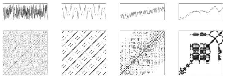
Typical examples of recurrence plots (top row: time series (plotted over time); bottom row: corresponding recurrence plots). From left to right: uncorrelated stochastic data (white noise), harmonic oscillation with two frequencies, chaotic data (logistic map) with linear trend, and data from an auto-regressive process.

The small-scale structures in recurrence plots contain information about certain characteristics of the dynamics of the underlying system. For example, the length of the diagonal lines visible in the recurrence plot are related to the divergence of phase space trajectories, thus, can represent information about the chaoticity ^[3] . Therefore, the recurrence quantification analysis quantifies the distribution of these small-scale structures ^{[4] [5] [6]} . This quantification can be used to describe the recurrence plots in a quantitative way. Applications are classification, predictions, nonlinear parameter estimation, and transition analysis. In contrast to the heuristic approach of the recurrence quantification analysis, which depends on the choice of the embedding parameters, some dynamical invariants as correlation dimension, K2 entropy or mutual information, which are independent on the embedding, can also be derived from recurrence plots. The base for these dynamical invariants are the recurrence rate and the distribution of the lengths of the diagonal lines ^[3] . More recent applications use recurrence plots as a tool for time series imaging in machine learning approaches and studying spatio-temporal recurrences ^[2] .

Close returns plots are similar to recurrence plots. The difference is that the relative time between recurrences is used for the ${\displaystyle y}$-axis (instead of absolute time) ^[6] .

The main advantage of recurrence plots is that they provide useful information even for short and non-stationary data, where other methods fail.

Extensions

Multivariate extensions of recurrence plots were developed as cross recurrence plots and joint recurrence plots.

Cross recurrence plots consider the phase space trajectories of two different systems in the same phase space ^[7] :

${\displaystyle \mathbf {CR} (i,j)=\Theta (\varepsilon -\|{\vec {x}}(i)-{\vec {y}}(j)\|),\quad {\vec {x}}(i),\,{\vec {y}}(i)\in \mathbb {R} ^{m},\quad i=1,\dots ,N_{x},\ j=1,\dots ,N_{y}.}$

The dimension of both systems must be the same, but the number of considered states (i.e. data length) can be different. Cross recurrence plots compare the occurrences of similar states of two systems. They can be used in order to analyse the similarity of the dynamical evolution between two different systems, to look for similar matching patterns in two systems, or to study the time-relationship of two similar systems, whose time-scale differ ^[8] .

Joint recurrence plots are the Hadamard product of the recurrence plots of the considered sub-systems ^[9] , e.g. for two systems ${\displaystyle {\vec {x}}}$ and ${\displaystyle {\vec {y}}}$ the joint recurrence plot is

${\displaystyle \mathbf {JR} (i,j)=\Theta (\varepsilon _{x}-\|{\vec {x}}(i)-{\vec {x}}(j)\|)\cdot \Theta (\varepsilon _{y}-\|{\vec {y}}(i)-{\vec {y}}(j)\|),\quad {\vec {x}}(i)\in \mathbb {R} ^{m},\quad {\vec {y}}(i)\in \mathbb {R} ^{n},\quad i,j=1,\dots ,N_{x,y}.}$

In contrast to cross recurrence plots, joint recurrence plots compare the simultaneous occurrence of recurrences in two (or more) systems. Moreover, the dimension of the considered phase spaces can be different, but the number of the considered states has to be the same for all the sub-systems. Joint recurrence plots can be used in order to detect phase synchronisation.

Example

Recurrence plot of the Southern Oscillation index.

See also

• Poincaré plot
• Recurrence period density entropy, an information-theoretic method for summarising the recurrence properties of both deterministic and stochastic dynamical systems.
• Recurrence quantification analysis, a heuristic approach to quantify recurrence plots.
• Self-similarity matrix
• Dot plot (bioinformatics)

References

1. J. P. Eckmann, S. O. Kamphorst, D. Ruelle (1987). "Recurrence Plots of Dynamical Systems". Europhysics Letters. 5 (9): 973–977. Bibcode:1987EL......4..973E. doi:10.1209/0295-5075/4/9/004. S2CID   250847435.
2. N. Marwan; K. H. Kraemer (2023). "Trends in recurrence analysis of dynamical systems". European Physical Journal ST. 232: 5–27. Bibcode:2023EPJST.232....5M. doi:10.1140/epjs/s11734-022-00739-8. S2CID   255630484.
3. N. Marwan; M. C. Romano; M. Thiel; J. Kurths (2007). "Recurrence Plots for the Analysis of Complex Systems". Physics Reports. 438 (5–6): 237. Bibcode:2007PhR...438..237M. doi:10.1016/j.physrep.2006.11.001.
4. J. P. Zbilut; C. L. Webber (1992). "Embeddings and delays as derived from quantification of recurrence plots". Physics Letters A. 171 (3–4): 199–203. Bibcode:1992PhLA..171..199Z. doi:10.1016/0375-9601(92)90426-M. S2CID   122890777.
5. C. L. Webber; J. P. Zbilut (1994). "Dynamical assessment of physiological systems and states using recurrence plot strategies". Journal of Applied Physiology. 76 (2): 965–973. doi:10.1152/jappl.1994.76.2.965. S2CID   23854540.
6. N. Marwan (2008). "A historical review of recurrence plots". European Physical Journal ST. 164 (1): 3–12. arXiv: 1709.09971 . Bibcode:2008EPJST.164....3M. doi:10.1140/epjst/e2008-00829-1. S2CID   119494395.
7. N. Marwan; J. Kurths (2002). "Nonlinear analysis of bivariate data with cross recurrence plots". Physics Letters A. 302 (5–6): 299–307. Bibcode:2002PhLA..302..299M. doi:10.1016/S0375-9601(02)01170-2. S2CID   8020903.
8. N. Marwan; J. Kurths (2005). "Line structures in recurrence plots". Physics Letters A. 336 (4–5): 349–357. Bibcode:2005PhLA..336..349M. doi:10.1016/j.physleta.2004.12.056. S2CID   931165.
9. M. C. Romano; M. Thiel; J. Kurths; W. von Bloh (2004). "Multivariate Recurrence Plots". Physics Letters A. 330 (3–4): 214–223. Bibcode:2004PhLA..330..214R. doi:10.1016/j.physleta.2004.07.066. S2CID   5746162.

External links

• Recurrence Plot