The method of least squares is a standard approach in regression analysis to approximate the solution of overdetermined systems by minimizing the sum of the squares of the residuals made in the results of each individual equation.
In mathematics, a Gaussian function, often simply referred to as a Gaussian, is a function of the form

In probability theory, a distribution is said to be stable if a linear combination of two independent random variables with this distribution has the same distribution, up to location and scale parameters. A random variable is said to be stable if its distribution is stable. The stable distribution family is also sometimes referred to as the Lévy alpha-stable distribution, after Paul Lévy, the first mathematician to have studied it.

The Gauss–Newton algorithm is used to solve non-linear least squares problems, which is equivalent to minimizing a sum of squared function values. It is an extension of Newton's method for finding a minimum of a non-linear function. Since a sum of squares must be nonnegative, the algorithm can be viewed as using Newton's method to iteratively approximate zeroes of the sum, and thus minimizing the sum. It has the advantage that second derivatives, which can be challenging to compute, are not required.

In probability theory and statistics, the inverse gamma distribution is a two-parameter family of continuous probability distributions on the positive real line, which is the distribution of the reciprocal of a variable distributed according to the gamma distribution.

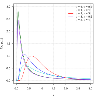
In probability theory and statistics, the generalized inverse Gaussian distribution (GIG) is a three-parameter family of continuous probability distributions with probability density function
In probability theory, the inverse Gaussian distribution is a two-parameter family of continuous probability distributions with support on (0,∞).
The scale space representation of a signal obtained by Gaussian smoothing satisfies a number of special properties, scale-space axioms, which make it into a special form of multi-scale representation. There are, however, also other types of "multi-scale approaches" in the areas of computer vision, image processing and signal processing, in particular the notion of wavelets. The purpose of this article is to describe a few of these approaches:
The normal-inverse Gaussian distribution (NIG) is a continuous probability distribution that is defined as the normal variance-mean mixture where the mixing density is the inverse Gaussian distribution. The NIG distribution was noted by Blaesild in 1977 as a subclass of the generalised hyperbolic distribution discovered by Ole Barndorff-Nielsen. In the next year Barndorff-Nielsen published the NIG in another paper. It was introduced in the mathematical finance literature in 1997.
In probability theory and statistics, the normal-gamma distribution is a bivariate four-parameter family of continuous probability distributions. It is the conjugate prior of a normal distribution with unknown mean and precision.

In probability theory and statistics, the half-normal distribution is a special case of the folded normal distribution.

In probability theory and statistics, the normal-inverse-gamma distribution is a four-parameter family of multivariate continuous probability distributions. It is the conjugate prior of a normal distribution with unknown mean and variance.
In numerical analysis Gauss–Laguerre quadrature is an extension of the Gaussian quadrature method for approximating the value of integrals of the following kind:
The generalized normal distribution or generalized Gaussian distribution (GGD) is either of two families of parametric continuous probability distributions on the real line. Both families add a shape parameter to the normal distribution. To distinguish the two families, they are referred to below as "symmetric" and "asymmetric"; however, this is not a standard nomenclature.
In probability and statistics, the K-distribution is a three-parameter family of continuous probability distributions. The distribution arises by compounding two gamma distributions. In each case, a re-parametrization of the usual form of the family of gamma distributions is used, such that the parameters are:

The multivariate stable distribution is a multivariate probability distribution that is a multivariate generalisation of the univariate stable distribution. The multivariate stable distribution defines linear relations between stable distribution marginals. In the same way as for the univariate case, the distribution is defined in terms of its characteristic function.

In fluid dynamics, a trochoidal wave or Gerstner wave is an exact solution of the Euler equations for periodic surface gravity waves. It describes a progressive wave of permanent form on the surface of an incompressible fluid of infinite depth. The free surface of this wave solution is an inverted (upside-down) trochoid – with sharper crests and flat troughs. This wave solution was discovered by Gerstner in 1802, and rediscovered independently by Rankine in 1863.
In mathematics, the Romanovski polynomials are one of three finite subsets of real orthogonal polynomials discovered by Vsevolod Romanovsky within the context of probability distribution functions in statistics. They form an orthogonal subset of a more general family of little-known Routh polynomials introduced by Edward John Routh in 1884. The term Romanovski polynomials was put forward by Raposo, with reference to the so-called 'pseudo-Jacobi polynomials in Lesky's classification scheme. It seems more consistent to refer to them as Romanovski–Routh polynomials, by analogy with the terms Romanovski–Bessel and Romanovski–Jacobi used by Lesky for two other sets of orthogonal polynomials.
Nonlinear mixed-effects models constitute a class of statistical models generalizing linear mixed-effects models. Like linear mixed-effects models, they are particularly useful in settings where there are multiple measurements within the same statistical units or when there are dependencies between measurements on related statistical units. Nonlinear mixed-effects models are applied in many fields including medicine, public health, pharmacology, and ecology.
The Kaniadakis logistic distribution is a generalized version of the logistic distribution associated with the Kaniadakis statistics. It is one example of a Kaniadakis distribution.