System dynamics

Dynamic stock and flow diagram of model New product adoption (model from article by John Sterman 2001 - True Software)

System dynamics (SD) is an approach to understanding the nonlinear behaviour of complex systems over time using stocks, flows, internal feedback loops, table functions and time delays. ^[1]

Overview

System dynamics is a methodology and mathematical modeling technique to frame, understand, and discuss complex issues and problems. Originally developed in the 1950s to help corporate managers improve their understanding of industrial processes, SD is currently being used throughout the public and private sector for policy analysis and design. ^[2]

Convenient graphical user interface (GUI) system dynamics software developed into user friendly versions by the 1990s and have been applied to diverse systems. SD models solve the problem of simultaneity (mutual causation) by updating all variables in small time increments with positive and negative feedbacks and time delays structuring the interactions and control. The best known SD model is probably the 1972 The Limits to Growth . This model forecast that exponential growth of population and capital, with finite resource sources and sinks and perception delays, would lead to economic collapse during the 21st century under a wide variety of growth scenarios.

System dynamics is an aspect of systems theory as a method to understand the dynamic behavior of complex systems. The basis of the method is the recognition that the structure of any system, the many circular, interlocking, sometimes time-delayed relationships among its components, is often just as important in determining its behavior as the individual components themselves. Examples are chaos theory and social dynamics. It is also claimed that because there are often properties-of-the-whole which cannot be found among the properties-of-the-elements, in some cases the behavior of the whole cannot be explained in terms of the behavior of the parts.

History

System dynamics was created during the mid-1950s ^[3] by Professor Jay Forrester of the Massachusetts Institute of Technology. In 1956, Forrester accepted a professorship in the newly formed MIT Sloan School of Management. His initial goal was to determine how his background in science and engineering could be brought to bear, in some useful way, on the core issues that determine the success or failure of corporations. Forrester's insights into the common foundations that underlie engineering, which led to the creation of system dynamics, were triggered, to a large degree, by his involvement with managers at General Electric (GE) during the mid-1950s. At that time, the managers at GE were perplexed because employment at their appliance plants in Kentucky exhibited a significant three-year cycle. The business cycle was judged to be an insufficient explanation for the employment instability. From hand simulations (or calculations) of the stock-flow-feedback structure of the GE plants, which included the existing corporate decision-making structure for hiring and layoffs, Forrester was able to show how the instability in GE employment was due to the internal structure of the firm and not to an external force such as the business cycle. These hand simulations were the start of the field of system dynamics. ^[2]

During the late 1950s and early 1960s, Forrester and a team of graduate students moved the emerging field of system dynamics from the hand-simulation stage to the formal computer modeling stage. Richard Bennett created the first system dynamics computer modeling language called SIMPLE (Simulation of Industrial Management Problems with Lots of Equations) in the spring of 1958. In 1959, Phyllis Fox and Alexander Pugh wrote the first version of DYNAMO (DYNAmic MOdels), an improved version of SIMPLE, and the system dynamics language became the industry standard for over thirty years. Forrester published the first, and still classic, book in the field titled Industrial Dynamics in 1961. ^[2]

From the late 1950s to the late 1960s, system dynamics was applied almost exclusively to corporate/managerial problems. In 1968, however, an unexpected occurrence caused the field to broaden beyond corporate modeling. John F. Collins, the former mayor of Boston, was appointed a visiting professor of Urban Affairs at MIT. The result of the Collins-Forrester collaboration was a book titled Urban Dynamics. The Urban Dynamics model presented in the book was the first major non-corporate application of system dynamics. ^[2] . In 1967, Richard M. Goodwin published the first edition of his paper "A Growth Cycle" ^[4] , which was the first attempt to apply the principles of system dynamics to economics. He devoted most of his life teaching what he called "Economic Dynamics", which could be considered a precursor of modern Non-equilibrium economics. ^[5]

The second major noncorporate application of system dynamics came shortly after the first. In 1970, Jay Forrester was invited by the Club of Rome to a meeting in Bern, Switzerland. The Club of Rome is an organization devoted to solving what its members describe as the "predicament of mankind"—that is, the global crisis that may appear sometime in the future, due to the demands being placed on the Earth's carrying capacity (its sources of renewable and nonrenewable resources and its sinks for the disposal of pollutants) by the world's exponentially growing population. At the Bern meeting, Forrester was asked if system dynamics could be used to address the predicament of mankind. His answer, of course, was that it could. On the plane back from the Bern meeting, Forrester created the first draft of a system dynamics model of the world's socioeconomic system. He called this model WORLD1. Upon his return to the United States, Forrester refined WORLD1 in preparation for a visit to MIT by members of the Club of Rome. Forrester called the refined version of the model WORLD2. Forrester published WORLD2 in a book titled World Dynamics. ^[2]

Topics in systems dynamics

The primary elements of system dynamics diagrams are feedback, accumulation of flows into stocks and time delays.

As an illustration of the use of system dynamics, imagine an organisation that plans to introduce an innovative new durable consumer product. The organisation needs to understand the possible market dynamics in order to design marketing and production plans.

Causal loop diagrams

Main article: Causal loop diagram

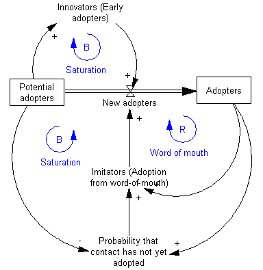
In the system dynamics methodology, a problem or a system (e.g., ecosystem, political system or mechanical system) may be represented as a causal loop diagram. ^[6] A causal loop diagram is a simple map of a system with all its constituent components and their interactions. By capturing interactions and consequently the feedback loops (see figure below), a causal loop diagram reveals the structure of a system. By understanding the structure of a system, it becomes possible to ascertain a system's behavior over a certain time period. ^[7]

The causal loop diagram of the new product introduction may look as follows:

Causal loop diagram of New product adoption model

There are two feedback loops in this diagram. The positive reinforcement (labeled R) loop on the right indicates that the more people have already adopted the new product, the stronger the word-of-mouth impact. There will be more references to the product, more demonstrations, and more reviews. This positive feedback should generate sales that continue to grow.

The second feedback loop on the left is negative reinforcement (or "balancing" and hence labeled B). Clearly, growth cannot continue forever, because as more and more people adopt, there remain fewer and fewer potential adopters.

Both feedback loops act simultaneously, but at different times they may have different strengths. Thus one might expect growing sales in the initial years, and then declining sales in the later years. However, in general a causal loop diagram does not specify the structure of a system sufficiently to permit determination of its behavior from the visual representation alone. ^[8]

Stock and flow diagrams

Main article: Stock and flow

Causal loop diagrams aid in visualizing a system's structure and behavior, and analyzing the system qualitatively. To perform a more detailed quantitative analysis, a causal loop diagram is transformed to a stock and flow diagram. A stock and flow model helps in studying and analyzing the system in a quantitative way; such models are usually built and simulated using computer software.

A stock is the term for any entity that accumulates or depletes over time. A flow is the rate of change in a stock.

A flow is the rate of accumulation of the stock

In this example, there are two stocks: Potential adopters and Adopters. There is one flow: New adopters. For every new adopter, the stock of potential adopters declines by one, and the stock of adopters increases by one.

Stock and flow diagram of New product adoption model

Equations

The real power of system dynamics is utilised through simulation. Although it is possible to perform the modeling in a spreadsheet, there are a variety of software packages that have been optimised for this.

The steps involved in a simulation are:

• Define the problem boundary
• Identify the most important stocks and flows that change these stock levels
• Identify sources of information that impact the flows
• Identify the main feedback loops
• Draw a causal loop diagram that links the stocks, flows and sources of information
• Write the equations that determine the flows
• Estimate the parameters and initial conditions. These can be estimated using statistical methods, expert opinion, market research data or other relevant sources of information. ^[9]
• Simulate the model and analyse results.

In this example, the equations that change the two stocks via the flow are:

${\displaystyle \ {\mbox{Potential adopters}}=-\int _{0}^{t}{\mbox{New adopters }}\,dt}$${\displaystyle \ {\mbox{Adopters}}=\int _{0}^{t}{\mbox{New adopters }}\,dt}$

Equations in discrete time

List of all the equations in discrete time, in their order of execution in each year, for years 1 to 15 :

${\displaystyle 1)\ {\mbox{Probability that contact has not yet adopted}}={\mbox{Potential adopters}}/({\mbox{Potential adopters }}+{\mbox{ Adopters}})}$${\displaystyle 2)\ {\mbox{Imitators}}=q\cdot {\mbox{Adopters}}\cdot {\mbox{Probability that contact has not yet adopted}}}$${\displaystyle 3)\ {\mbox{Innovators}}=p\cdot {\mbox{Potential adopters}}}$${\displaystyle 4)\ {\mbox{New adopters}}={\mbox{Innovators}}+{\mbox{Imitators}}}$${\displaystyle 4.1)\ {\mbox{Potential adopters}}\ -={\mbox{New adopters }}}$${\displaystyle 4.2)\ {\mbox{Adopters}}\ +={\mbox{New adopters }}}$

${\displaystyle \ p=0.03}$${\displaystyle \ q=0.4}$

Dynamic simulation results

Main article: Dynamic simulation

The dynamic simulation results show that the behaviour of the system would be to have growth in adopters that follows a classic s-curve shape.
The increase in adopters is very slow initially, then exponential growth for a period, followed ultimately by saturation.

Dynamic stock and flow diagram of New product adoption model

Stocks and flows values for years = 0 to 15

Equations in continuous time

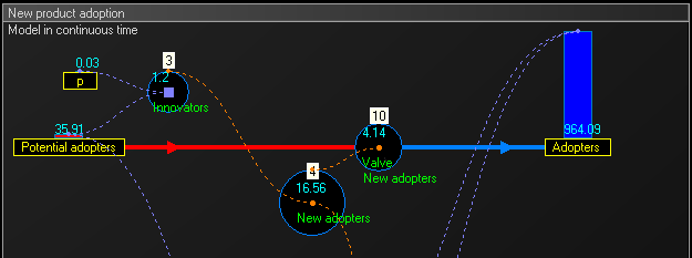
To get intermediate values and better accuracy, the model can run in continuous time: we multiply the number of units of time and we proportionally divide values that change stock levels. In this example we multiply the 15 years by 4 to obtain 60 quarters, and we divide the value of the flow by 4.
Dividing the value is the simplest with the Euler method, but other methods could be employed instead, such as Runge–Kutta methods.

List of the equations in continuous time for trimesters = 1 to 60 :

• They are the same equations as in the section Equation in discrete time above, except equations 4.1 and 4.2 replaced by following :

${\displaystyle 10)\ {\mbox{Valve New adopters}}\ ={\mbox{New adopters}}\cdot TimeStep}$${\displaystyle 10.1)\ {\mbox{Potential adopters}}\ -={\mbox{Valve New adopters}}}$${\displaystyle 10.2)\ {\mbox{Adopters}}\ +={\mbox{Valve New adopters }}}$

${\displaystyle \ TimeStep=1/4}$

• In the below stock and flow diagram, the intermediate flow 'Valve New adopters' calculates the equation :

${\displaystyle \ {\mbox{Valve New adopters}}\ ={\mbox{New adopters }}\cdot TimeStep}$

Dynamic stock and flow diagram of New product adoption model in continuous time

Application

System dynamics has found application in a wide range of areas, for example population, agriculture, ^[10] ecological and economic systems, which usually interact strongly with each other.

System dynamics have various "back of the envelope" management applications. They are a potent tool to:

• Teach system thinking reflexes to persons being coached
• Analyze and compare assumptions and mental models about the way things work
• Gain qualitative insight into the workings of a system or the consequences of a decision
• Recognize archetypes of dysfunctional systems in everyday practice

Computer software is used to simulate a system dynamics model of the situation being studied. Running "what if" simulations to test certain policies on such a model can greatly aid in understanding how the system changes over time. System dynamics is very similar to systems thinking and constructs the same causal loop diagrams of systems with feedback. However, system dynamics typically goes further and utilises simulation to study the behaviour of systems and the impact of alternative policies. ^[11]

System dynamics has been used to investigate resource dependencies, and resulting problems, in product development. ^{[12] [13]}

A system dynamics approach to macroeconomics, known as Minsky , has been developed by the economist Steve Keen. ^[14] This has been used to successfully model world economic behaviour from the apparent stability of the Great Moderation to the sudden unexpected Financial crisis of 2007–08.

Example: Growth and decline of companies

Causal loop diagram of a model examining the growth or decline of a life insurance company.

The figure above is a causal loop diagram of a system dynamics model created to examine forces that may be responsible for the growth or decline of life insurance companies in the United Kingdom. A number of this figure's features are worth mentioning. The first is that the model's negative feedback loops are identified by C's, which stand for Counteracting loops. The second is that double slashes are used to indicate places where there is a significant delay between causes (i.e., variables at the tails of arrows) and effects (i.e., variables at the heads of arrows). This is a common causal loop diagramming convention in system dynamics. Third, is that thicker lines are used to identify the feedback loops and links that author wishes the audience to focus on. This is also a common system dynamics diagramming convention. Last, it is clear that a decision maker would find it impossible to think through the dynamic behavior inherent in the model, from inspection of the figure alone. ^[15]

Example: Piston motion

1. Objective: study of a crank-connecting rod system.
   We want to model a crank-connecting rod system through a system dynamic model. Two different full descriptions of the physical system with related systems of equations can be found here (in English) and here (in French); they give the same results. In this example, the crank, with variable radius and angular frequency, will drive a piston with a variable connecting rod length.
2. System dynamic modeling: the system is now modeled, according to a stock and flow system dynamic logic.
   The figure below shows the stock and flow diagram

   

   Stock and flow diagram for crank-connecting rod system

3. Simulation: the behavior of the crank-connecting rod dynamic system can then be simulated.
   The next figure is a 3D simulation created using procedural animation. Variables of the model animate all parts of this animation: crank, radius, angular frequency, rod length, and piston position.

3D procedural animation of the crank-connecting rod system modeled in 2

See also

Related subjects Causal loop diagram Comparison of system dynamics software Ecosystem model Plateau Principle System archetypes System Dynamics Society Twelve leverage points Wicked problems World3 Population dynamics Predator-prey interaction

Related fields Dynamical systems theory Grey box model Operations research Social dynamics System identification Systems theory Systems thinking TRIZ

Related scientists Jay Forrester Dennis Meadows Donella Meadows Peter Senge Graeme Snooks John Sterman

Systems science portal

References

1. "MIT System Dynamics in Education Project (SDEP)".
2. Michael J. Radzicki and Robert A. Taylor (2008). "Origin of System Dynamics: Jay W. Forrester and the History of System Dynamics". In: U.S. Department of Energy's Introduction to System Dynamics. Retrieved 23 October 2008.
3. Forrester, Jay (1971). Counterintuitive behavior of social systems. Technology Review 73(3): 52–68
4. Goodwin, R.M. (1982). A Growth Cycle. In: Essays in Economic Dynamics. Palgrave Macmillan, London.
5. Di Matteo, M., & Sordi, S. (2015). Goodwin in Siena: economist, social philosopher and artist. Cambridge Journal of Economics, 39(6), 1507–1527.
6. Sterman, John D. (2000). Business Dynamics: Systems Thinking and Modeling for a Complex World. Boston: McGraw-Hill. ISBN   0-07-231135-5.
7. Meadows, Donella. (2008). Thinking in Systems: A Primer. Earthscan
8. Richardson, G. P. (1986). "Problems with causal-loop diagrams". Syst. Dyn. Rev. 2 (2): 158–170. doi:10.1002/sdr.4260020207.
9. Sterman, John D. (2001). "System dynamics modeling: Tools for learning in a complex world". California Management Review. 43 (4): 8–25. doi:10.2307/41166098. JSTOR   41166098. S2CID   4637381.
10. F. H. A. Rahim, N. N. Hawari and N. Z. Abidin, "Supply and demand of rice in Malaysia: A system dynamics approach", International Journal of Supply Chain and Management, Vol.6, No.4, pp. 234-240, 2017.
11. System Dynamics Society
12. Repenning, Nelson P. (2001). "Understanding fire fighting in new product development" (PDF). The Journal of Product Innovation Management. 18 (5): 285–300. doi:10.1016/S0737-6782(01)00099-6. hdl: 1721.1/3961 .
13. Nelson P. Repenning (1999). Resource dependence in product development improvement efforts, MIT Sloan School of Management Department of Operations Management/System Dynamics Group, Dec 1999.
14.    Minsky - Project of the month January 2014. Interview with Minsky development team. Accessed January 2014
15. 1 2 Michael J. Radzicki and Robert A. Taylor (2008). "Feedback". In: U.S. Department of Energy's Introduction to System Dynamics. Retrieved 23 October 2008.

Further reading

• Kypuros, Javier (2013). System dynamics and control with bond graph modeling. Boca Raton: Taylor & Francis. ISBN   978-1466560758.
• Forrester, Jay W. (1961). Industrial Dynamics. Pegasus Communications. ISBN   978-1-883823-36-8.
• Forrester, Jay W. (1969). Urban Dynamics. Pegasus Communications. ISBN   978-1-883823-39-9.
• Meadows, Donella H. (1972). Limits to Growth. New York: University books. ISBN   978-0-87663-165-2.
• Morecroft, John (2007). Strategic Modelling and Business Dynamics: A Feedback Systems Approach. John Wiley & Sons. ISBN   978-0-470-01286-4.
• Roberts, Edward B. (1978). Managerial Applications of System Dynamics . Cambridge: MIT Press. ISBN   978-0-262-18088-7.
• Randers, Jorgen (1980). Elements of the System Dynamics Method. Cambridge: MIT Press. ISBN   978-0-915299-39-3.
• Senge, Peter (1990). The Fifth Discipline. Currency. ISBN   978-0-385-26095-4.
• Sterman, John D. (2000). Business Dynamics: Systems thinking and modeling for a complex world. McGraw Hill. ISBN   978-0-07-231135-8.

External links

• System Dynamics Society
• Study Prepared for the U.S. Department of Energy's Introducing System Dynamics -
• Desert Island Dynamics "An Annotated Survey of the Essential System Dynamics Literature"
• True World : Temporal Reasoning Universal Elaboration  : System Dynamics software used for diagrams in this article (free)