For the noises made by the human lung, see Crackles.
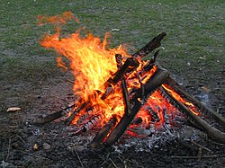
Burning wood produces a random crackling noise
Crackling noise arises when a system is subject to an external force and it responds via events that appear very similar at many different scales. In a classical system there are usually two states, on and off. However, sometimes a state can exist in between. There are three main categories this noise can be sorted into: the first is popping where events at very similar magnitude occur continuously and randomly, e.g. popcorn; the second is snapping where there is little change in the system until a critical threshold is surpassed, at which point the whole system flips from one state to another, e.g. snapping a pencil; the third is crackling which is a combination of popping and snapping, where there are some small and some large events with a relation law predicting their occurrences, referred to as universality.[1] Crackling can be observed in many natural phenomena, e.g. crumpling paper,[2] candy wrappers (or other elastic sheets),[3][4] fire, occurrences of earthquakes and the magnetisation of ferromagnetic material.
Cracking noise contrasts with snapping noise and popping noise. Snapping noise is one large yielding event, while popping noise is a constant level of similar-sized, small yielding events. Crackling is between these. It occurs when connection strengths between components of the system is at a critical level, such that there are many yielding events with sizes spanned across several orders of magnitude.[5]
Some of these systems are reversible, such as demagnetisation (by heating a magnet to its Curie temperature),[6] while others are irreversible, such as an avalanche (where the snow can only move down a mountain), but many systems have a positive bias causing it to eventually move from one state to another, such as gravity or another external force.
Theory
Barkhausen noise
Magnetization (J) or flux density (B) curve as a function of magnetic field intensity (H) in ferromagnetic material. The inset shows the jumps responsible for Barkhausen noise.
Research into the study of small perturbations within a large domains began in the late 1910s when Heinrich Barkhausen investigated how the domains, or dipoles, within a ferromagnetic material changed under the influence of an external magnetic field. When demagnetised, a magnet’s dipoles are pointing in random directions hence the net magnetic force from all the dipoles will be zero. By coiling an iron bar with wire and passing an electric current through the wire, a magnetic field perpendicular to the coil is produced (Fleming’s right hand rule for a coil), this causes the dipoles within the magnet to align to the external field.
Contrary to what was thought at the time that these domains flip continuously one by one, Barkhausen found that clusters of domains flipped in small discrete steps.[7] By coiling a secondary coil around the bar connected to a speaker or detector, when a cluster of domains change alignment a change in flux occurs, this disrupts the current in the secondary coil and hence causes a signal output. When played out loud, this is referred to as Barkhausen noise, the magnetisation of the magnet increases in discrete steps as a function of the flux density.[8]
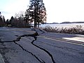
Further research into crackling noise was done in the late 1940s by Charles Francis Richter and Beno Gutenberg who examined earthquakes analytically. Before the invention of the well-known Richter scale, the Mercalli intensity scale was used; this is a subjective measurement of how damaging an earthquake was to property, i.e. II would be small vibrations and objects moving, while XII would be wide spread destruction of all buildings. The Richter scale is a logarithmic scale which measures the energy and amplitude of vibrations dissipated from the epicentre of the earthquake, i.e. a 7.0 earthquake is 10 times more powerful than a 6.0 earthquake. Together with Gutenberg, they went on to discover the Gutenberg–Richter law which is a probability distribution relationship between the magnitude of an earthquake and its probability of occurrence. It states that small earthquakes happen much more frequently and larger earthquakes occur very rarely.[9]
Gutenberg–Richter law[10] shows an inverse power relation between the number of earthquakes occurring N and its magnitude M with a proportionality constant b and intercepta.
Simulation
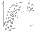
Evolution of a 2D Cellular Automaton simulation over time. Initially the system pops, then it crackles with some small and some large clusters turning white and remain white, finally the system snaps to a global positive state (+1).
To truly simulate such an environment, one would need a continuous infinite 3D system, however due to computational limitations a 2D cellular automata can be used to provide a near approximation; a million cells in the form of a 1000x1000 matrix is sufficient to test most scenarios. Each cell stores two pieces of information; the force applied to the cell which is a continuous quantity, and the state of the cell which is an integer value of either +1 (on) or −1 (off).
Parametrisation
The net force is composed of three components which can correspond to physical attributes of any crackling noise system; the first is an external force field (K) that increases with time (t). The second component is a force that is dependent on the sum of the states of neighbouring cells (S) and the third is a random component (r) scaled by (X)[11]
The external force K is multiplied by time (t), where K is a positive scalar constant, however this can be varying and or negative as well. S represents the state of a cell (+1 or −1), the second component takes the sum of the four neighbouring cell states (up, down, left & right) and multiplies it by another scalar quantity, this is analogous to a coupling constant (J). The random number generator (r) is a normally distributed range of values with a mean of zero and a fixed standard deviation (rσ), this is also multiplied by a scalar constant (X). Of the three components of the net force (F), the neighbour and random components can produce positive and negative values, while the external force is only positive meaning that there is a forward bias applied to the system which over time becomes the dominant force.
If the net force on a cell is positive it will turn the cell on (+1) and off (−1) if the force on the cell is negative. In a 2D system, there are a multitude of state combinations and arrangements possible, but this can be grouped into three regions, two global stable states of all +1s or all −1s and an unstable state in between where there is a mixture of both states. Traditionally if the system is unstable it will shortly flip to one of the global states, however under the perfect conditions, i.e. a critical point, a metastable state can form in between the two global states which is only sustainable if the parameters for the net force are balanced. The boundary conditions for the matrix wrap around top to bottom and left to right, problems for the corner cells can be negated using a large matrix.
Snap, crackle and pop
Three statements can be formed to describe when and how the system reacts to stimulus. The difference between the external field and the other components decides whether a system pops or crackles, but there is also a special case if the modulus of the random and neighbour components are much greater than the external field, the system snaps to a density of zero and then slows down its rate of conversion.
Popping is when there are small perturbations to the system which are reversible and have a negligible effect on the global system state.
Snapping is when large clusters of cells or the whole system flips to an alternate state, i.e. all +1s or all −1s. The whole system will only flip when it has reached a critical or tipping point.
Crackling is observed when the system experiences popping and snapping of reversible small and large clusters. The system is constantly imbalanced and attempts to reach equilibrium which is not possible due to internal or external forces.
Physical meaning of components
Random component (r)
By simulating earthquakes it is possible to observe the Gutenberg–Richter law, in this system the random component would have represented random perturbations in the ground and air and this could be anything from a violent weather system, natural continuous stimuli like a river flowing, waves hitting the shoreline or human activity such as drilling. This is much like the butterfly effect where one could not predict a future outcome of an event nor trace back to the original condition from a set time during the simulation and at the macroscopic level appears insignificant, but at the microscopic level may have been the cause for a chain reaction of events; one cell switching on may be responsible for the whole system flipping on.
Neighbour component (ΣS)
The neighbour component for physical objects such as rocks or tectonic plates is simply a description of Newton’s laws of motion, if a plate is moving and collides with another plate, the other plate will provide a reactionary force, similarly if a large collection of loose particles (boulders, faults) is forced against its neighbour, the adjacent particle/object will also move.
External force (K)
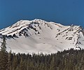
The external force are the long term movements of tectonic plates or the liquid rock currents within the upper mantle, which is a continuous force applied eventually the plate will snap back or fracture relieving stress on the system to flipping it to a stable state, i.e. an earthquake. Volcanoes are similar in that the build-up of magma pressure underneath will eventually overcome the layer of dry rock on top causing an eruption. Such models can be used to predict the occurrence of earthquakes and volcanoes in active regions and predict aftershocks which are common after a large events.
Practical applications
During magnetisation of a magnet; the external field is the applied electric field, the neighbour component is the effect of localised magnetic fields of the dipoles and the random component represents other perturbations from external or internal stimuli. There are many practical applications to this, a manufacturer can use this type of simulation to non-destructively test their magnets to see how it responds under certain conditions. To test its magnetisation after taking a large force i.e. a hammer blow or dropping it on the floor, one could suddenly increase the external force (H) or the coupling constant (J). To test heat conditions a boundary condition could be applied to one edge with an increase in thermal fluctuations (increase X), this would require a three dimensional model.
Business world
The behaviour of stock prices have shown properties of universality. By taking historical share price data of a company,[12] calculating the daily returns and then plotting this in a histogram would produce a fat-tailed non-Gaussian distribution. Stock prices will fluctuate with small variations constantly and larger changes much more rarely; a stock exchange could be interpreted as the force responsible to bring the share price to equilibrium by adjusting the price to the supply and demand quota.
The mergers of companies where small companies are regularly forming, often start-ups which are very volatile, if it survives a period of time then it is likely to continue to grow, once it becomes large enough it is able to buy other smaller companies increasing its own size. This is much like larger companies buying their competitors out to increase their own market share and so on and so forth, until the market becomes saturated.
Examples in the natural world
It is not possible for systems in the real world to remain in permanent equilibrium as there are too many external factors contributing to the system's state. The system can either be in temporary equilibrium and then suddenly fail due to a stimulus or be in a constant state of changing phases due to an external force attempting to balance the system. These systems observe popping, snapping and crackling behaviour.
Sunspot number over time. Dataset from NOAA. It starts on 1945-01-01 and ends on 2017-06-30. The number of each day is converted to an audio pulse with that amplitude, 0.01 seconds long.
Frequency of earthquakes as a function of earthquake magnitude (Gutenberg–Richter law).
The rate at which a ferromagnetic bar's domain aligns to an external magnetic field creates the Barkhausen effect.
The sound of corn popping is an instance of popping, not crackling.[5]
The size distribution of avalanche due to excess snow build up spans several orders of magnitude.[13]
The snapping of a pencil due to inelastic mechanical properties of the wood is an instance of snapping, not crackling.[5]
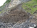
The distribution of landslides is a crackling noise, spanning from collapse of a molehill to collapse of a mountainside.
A volcano will eventually erupt when the pressure build up of internal magma flow is greater than the seal.
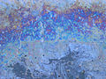
Van der Waals forces mean that fat globules forming on the surface of water will attract to one another to reduce the free energy and become larger clusters
↑ Schroder, Malte (2013). Crackling Noise in Fractional Percolation – Randomly distributed discontinuous jumps in explosive percolation. Max Planck Institute for Dynamics & Self-Organization.
This page is based on this Wikipedia article Text is available under the CC BY-SA 4.0 license; additional terms may apply. Images, videos and audio are available under their respective licenses.