The propagation constant of a sinusoidal electromagnetic wave is a measure of the change undergone by the amplitude and phase of the wave as it propagates in a given direction. The quantity being measured can be the voltage, the current in a circuit, or a field vector such as electric field strength or flux density. The propagation constant itself measures the change per unit length, but it is otherwise dimensionless. In the context of two-port networks and their cascades, propagation constant measures the change undergone by the source quantity as it propagates from one port to the next.

In the mathematical field of differential geometry, the Riemann curvature tensor or Riemann–Christoffel tensor is the most common way used to express the curvature of Riemannian manifolds. It assigns a tensor to each point of a Riemannian manifold. It is a local invariant of Riemannian metrics which measures the failure of the second covariant derivatives to commute. A Riemannian manifold has zero curvature if and only if it is flat, i.e. locally isometric to the Euclidean space. The curvature tensor can also be defined for any pseudo-Riemannian manifold, or indeed any manifold equipped with an affine connection.

Flight dynamics is the science of air vehicle orientation and control in three dimensions. The three critical flight dynamics parameters are the angles of rotation in three dimensions about the vehicle's center of gravity (cg), known as pitch, roll and yaw.
In the calculus of variations, a field of mathematical analysis, the functional derivative relates a change in a Functional to a change in a function on which the functional depends.

In thermodynamics, the Onsager reciprocal relations express the equality of certain ratios between flows and forces in thermodynamic systems out of equilibrium, but where a notion of local equilibrium exists.

In applied mechanics, bending characterizes the behavior of a slender structural element subjected to an external load applied perpendicularly to a longitudinal axis of the element.
In mathematics, in particular in algebraic geometry and differential geometry, Dolbeault cohomology is an analog of de Rham cohomology for complex manifolds. Let M be a complex manifold. Then the Dolbeault cohomology groups depend on a pair of integers p and q and are realized as a subquotient of the space of complex differential forms of degree (p,q).
A quasiprobability distribution is a mathematical object similar to a probability distribution but which relaxes some of Kolmogorov's axioms of probability theory. Quasiprobabilities share several of general features with ordinary probabilities, such as, crucially, the ability to yield expectation values with respect to the weights of the distribution. They can however violate the σ-additivity axiom: integrating them over does not necessarily yield probabilities of mutually exclusive states. Indeed, quasiprobability distributions also counterintuitively have regions of negative probability density, contradicting the first axiom. Quasiprobability distributions arise naturally in the study of quantum mechanics when treated in phase space formulation, commonly used in quantum optics, time-frequency analysis, and elsewhere.

The covariant formulation of classical electromagnetism refers to ways of writing the laws of classical electromagnetism in a form that is manifestly invariant under Lorentz transformations, in the formalism of special relativity using rectilinear inertial coordinate systems. These expressions both make it simple to prove that the laws of classical electromagnetism take the same form in any inertial coordinate system, and also provide a way to translate the fields and forces from one frame to another. However, this is not as general as Maxwell's equations in curved spacetime or non-rectilinear coordinate systems.
In physics, Maxwell's equations in curved spacetime govern the dynamics of the electromagnetic field in curved spacetime or where one uses an arbitrary coordinate system. These equations can be viewed as a generalization of the vacuum Maxwell's equations which are normally formulated in the local coordinates of flat spacetime. But because general relativity dictates that the presence of electromagnetic fields induce curvature in spacetime, Maxwell's equations in flat spacetime should be viewed as a convenient approximation.
There are various mathematical descriptions of the electromagnetic field that are used in the study of electromagnetism, one of the four fundamental interactions of nature. In this article, several approaches are discussed, although the equations are in terms of electric and magnetic fields, potentials, and charges with currents, generally speaking.
In probability theory and statistics, the Dirichlet-multinomial distribution is a family of discrete multivariate probability distributions on a finite support of non-negative integers. It is also called the Dirichlet compound multinomial distribution (DCM) or multivariate Pólya distribution. It is a compound probability distribution, where a probability vector p is drawn from a Dirichlet distribution with parameter vector , and an observation drawn from a multinomial distribution with probability vector p and number of trials n. The Dirichlet parameter vector captures the prior belief about the situation and can be seen as a pseudocount: observations of each outcome that occur before the actual data is collected. The compounding corresponds to a Pólya urn scheme. It is frequently encountered in Bayesian statistics, machine learning, empirical Bayes methods and classical statistics as an overdispersed multinomial distribution.
A ratio distribution is a probability distribution constructed as the distribution of the ratio of random variables having two other known distributions. Given two random variables X and Y, the distribution of the random variable Z that is formed as the ratio Z = X/Y is a ratio distribution.

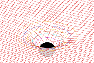
In general relativity, a point mass deflects a light ray with impact parameter by an angle approximately equal to
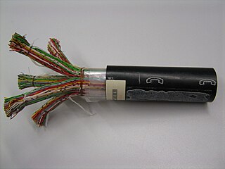
The primary line constants are parameters that describe the characteristics of conductive transmission lines, such as pairs of copper wires, in terms of the physical electrical properties of the line. The primary line constants are only relevant to transmission lines and are to be contrasted with the secondary line constants, which can be derived from them, and are more generally applicable. The secondary line constants can be used, for instance, to compare the characteristics of a waveguide to a copper line, whereas the primary constants have no meaning for a waveguide.
In continuum mechanics, a compatible deformation tensor field in a body is that unique tensor field that is obtained when the body is subjected to a continuous, single-valued, displacement field. Compatibility is the study of the conditions under which such a displacement field can be guaranteed. Compatibility conditions are particular cases of integrability conditions and were first derived for linear elasticity by Barré de Saint-Venant in 1864 and proved rigorously by Beltrami in 1886.

The Kirchhoff–Love theory of plates is a two-dimensional mathematical model that is used to determine the stresses and deformations in thin plates subjected to forces and moments. This theory is an extension of Euler-Bernoulli beam theory and was developed in 1888 by Love using assumptions proposed by Kirchhoff. The theory assumes that a mid-surface plane can be used to represent a three-dimensional plate in two-dimensional form.
A product distribution is a probability distribution constructed as the distribution of the product of random variables having two other known distributions. Given two statistically independent random variables X and Y, the distribution of the random variable Z that is formed as the product
In mathematics, infinite compositions of analytic functions (ICAF) offer alternative formulations of analytic continued fractions, series, products and other infinite expansions, and the theory evolving from such compositions may shed light on the convergence/divergence of these expansions. Some functions can actually be expanded directly as infinite compositions. In addition, it is possible to use ICAF to evaluate solutions of fixed point equations involving infinite expansions. Complex dynamics offers another venue for iteration of systems of functions rather than a single function. For infinite compositions of a single function see Iterated function. For compositions of a finite number of functions, useful in fractal theory, see Iterated function system.
In mathematics, Ricci calculus constitutes the rules of index notation and manipulation for tensors and tensor fields on a differentiable manifold, with or without a metric tensor or connection. It is also the modern name for what used to be called the absolute differential calculus, developed by Gregorio Ricci-Curbastro in 1887–1896, and subsequently popularized in a paper written with his pupil Tullio Levi-Civita in 1900. Jan Arnoldus Schouten developed the modern notation and formalism for this mathematical framework, and made contributions to the theory, during its applications to general relativity and differential geometry in the early twentieth century.


