This article is being considered for deletion in accordance with Wikipedia's deletion policy. Please share your thoughts on the matter at this article's deletion discussion page. |
This article needs attention from an expert in Physics. The specific problem is: Needs to be integrated with existing physics coverage..(December 2014) |
The electrokinematics theorem [1] [2] [3] connects the velocity and the charge of carriers moving inside an arbitrary volume to the currents, voltages and power on its surface through an arbitrary irrotational vector. Since it contains, as a particular application, the Ramo-Shockley theorem, [4] [5] the electrokinematics theorem is also known as Ramo-Shockly-Pellegrini theorem.
To introduce the electrokinematics theorem let us first list a few definitions: qj, rj and vj are the electric charge, position and velocity, respectively, at the time t of the jth charge carrier; , and are the electric potential, field, and permittivity, respectively, , and are the conduction, displacement and, in a 'quasi-electrostatic' assumption, total current density, respectively; is an arbitrary irrotational vector in an arbitrary volume enclosed by the surface S, with the constraint that . Now let us integrate over the scalar product of the vector by the two members of the above-mentioned current equation. Indeed, by applying the divergence theorem, the vector identity , the above-mentioned constraint and the fact that , we obtain the electrokinematics theorem in the first form
which, taking into account the corpuscular nature of the current , where is the Dirac delta function and N(t) is the carrier number in at the time t, becomes
A component of the total electric potential is due to the voltage applied to the kth electrode on S, on which (and with the other boundary conditions on the other electrodes and for ), and each component is due to the jth charge carrier qj , being for and over any electrode and for . Moreover, let the surface S enclosing the volume consist of a part covered by n electrodes and an uncovered part .
According to the above definitions and boundary conditions, and to the superposition theorem, the second equation can be split into the contributions
relative to the carriers and to the electrode voltages, respectively, being the total number of carriers in the space, inside and outside , at time t, and . The integrals of the above equations account for the displacement current, in particular across .
One of the more meaningful application of the above equations is to compute the current
through an hth electrode of interest corresponding to the surface , and being the current due to the carriers and to the electrode voltages, to be computed through third and fourth equations, respectively.
Consider as a first example, the case of a surface S that is not completely covered by electrodes, i.e., , and let us choose Dirichlet boundary conditions on the hth electrode of interest and of on the other electrodes so that, from the above equations we have
where is relative to the above-mentioned boundary conditions and is a capacitive coefficient of the hth electrode given by
is the voltage difference between the hth electrode and an electrode held to a constant voltage (DC), for instance, directly connected to ground or through a DC voltage source. The above equations hold true for the above Dirichlet conditions for and for any other choice of boundary conditions on .
A second case can be that in which also on so that such equations reduce to
As a third case, exploiting also to the arbitrariness of , we can choose a Neumann boundary condition of tangent to in any point. Then the equations become
In particular, this case is useful when the device is a right parallelepiped, being and the lateral surface and the bases, respectively.
As a fourth application let us assume in the whole the volume , i.e., in it, so that from the first equation of Section 1 we have
which recover the Kirchhoff law with the inclusion the displacement current across the surface that is not covered by electrodes.
A fifth case, historically significant, is that of electrodes that completely enclose the volume of the device, i.e. . Indeed, choosing again the Dirichlet boundary conditions of on and on the other electrodes, from the equations for the open device we get the relationships
with
thus obtaining the Ramo-Shockly theorem as a particular application of the electrokinematics theorem, extended from the vacuum devices to any electrical component and material.
As the above relationships hold true also when depends on time, we can have a sixty application if we select as the electric field generated by the electrode voltages when there is no charge in . Indeed, as the first equation can be written in the form
from which we have
where corresponds to the power entering the device across the electrodes (enclosing it). On the other side
gives the increment of the internal energy in in a unit of time, being the total electric field of which is due to the electrodes and is due to the whole charge density in with over S. Then it is , so that, according to such equations, we also verify the energy balance by means of the electrokinematics theorem. With the above relationships the balance can be extended also to the open devices by taking into account the displacement current across .
A meaningful application of the above results is also the computation of the fluctuations of the current when the electrode voltages is constant, because this is useful for the evaluation of the device noise. To this end, we can exploit the first equation of section Open devices, because it concerns the more general case of an open device and it can be reduced to a more simply relationship. This happens for frequencies , ( being the transit time of the jth carrier across the device) because the in time integral of the above equation of the Fourier transform to be performed to compute the power spectral density (PSD) of the noise, the time derivatives provides no contribution. Indeed, according to the Fourier transform, this result derives from integrals such as , in which . Therefore, for the PSD computation we can exploit the relationships
Moreover, as it can be shown, [6] this happens also for , for instance when the jth carrier is stored for a long time in a trap if the screening length due to the other carriers is small in comparison to size. All the above considerations hold true for any size of , including nanodevices. In particular we have a meaningful case when the device is a right parallelepiped or cylinder with as lateral surface and u as the unit vector along its axis, with the bases and located at a distance L as electrodes, and with . Indeed, choosing , from the above equation we finally obtain the current ,
where and are the components of and along . The above equations in their corpuscular form are particularly suitable for the investigation of transport and noise phenomena from the microscopic point of view, with the application of both the analytical approaches and numerical statistical methods, such as the Monte Carlo techniques. On the other side, in their collective form of the last terms, they are useful to connect, with a general and new method, the local variations of continuous quantities to the current fluctuation at the device terminals. This will be shown in the next sections.
Let us first evaluate the PSD of the shot noise of the current for short circuited device terminals, i.e. when the 's are constant, by applying the third member of the first equation of the above Section. To this end, let us exploit the Fourier coefficient
and the relationship
where , in the second term and in the third. If we define with and the beginning and the end of the jth carrier motion inside , we have either and or vice versa (the case of give no contribution), so that from the first equations of the above and of this Section, we get
where is the number of the carriers (with equal charge q) that start from (arrive on) the electrode of interest during the time interval . Finally for , being the correlation time, and for carriers with a motion that is statistically independent and a Poisson process we have , and so that we obtain
where is the average current due to the carriers leaving (reaching) the electrode. Therefore, we recover and extend the Schottky's theorem [7] on shot noise. For instance for an ideal pn junction, or Schottky barrier diode, it is , , where is the Boltzmann constant, T the absolute temperature, v the voltage and the total current. In particular, for the conductance becomes and the above equation gives
that is the thermal noise at thermal equilibrium given by the Nyquist theorem. [8] If the carrier motions are correlated, the above equation has to be changed to the form (for )
where is the so-called Fano factor that can be both less than 1 (for instance in the case of carrier generation-recombination in nonideal pn junctions [9] ), and greater than 1 (as in the negative resistance region of resonant-tunneling diode, as a result of the electron-electron interaction being enhanced by the particular shape of the density of states in the well. [2] [10] )
Once again from the corpuscular point of view, let us evaluate the thermal noise with the autocorrelation function of by means of the second term of the second equation of section Fluctuations, that for the short circuit condition (i.e., at thermal equilibrium) which implies , becomes
where m is the carrier effective mass and . As and are the carrier mobility and the conductance of the device, from the above equation and the Wiener–Khinchin theorem [11] [12] we recover the result
obtained by Nyquist from the second principle of the thermodynamics, i.e. by means of a macroscopic approach. [8]
A significant example of application of the macroscopic point of view expressed by the third term of the second equation of section Fluctuations is represented by the g-r noise generated by the carrier trapping-detrapping processes in device defects. In the case of constant voltages and drift current density , that is by neglecting the above velocity fluctuations of thermal origin, from the mentioned equation we get
in which is the carrier density, and its steady state value is , being the device cross-section surface; furthermore, we use the same symbols for both the time averaged and the instantaneous quantities. Let us first evaluate the fluctuations of the current i, that from the above equation are
where only the fluctuation terms are time dependent. The mobility fluctuations can be due to the motion or to the change of status of defects that we neglect here. Therefore, we ascribe the origin of g-r noise to the trapping-detrapping processes that contribute to through the other two terms via the fluctuation of the electron number in the energy level of a single trap in the channel or in its neighborhood. Indeed, the charge fluctuation in the trap generates variations of and of . However, the variation does not contribute to because it is odd in the u direction, so that we get
from which we obtain
where the reduction of the integration volume from to the much smaller one around the defect is justified by the fact that the effects of and fade within a few multiples of a screening length, which can be small (of the order of nanometers [7] in graphene [11] ); from Gauss's theorem, we obtain also and the r.h.s. of the equation. In it the variation occurs around the average value given by the Fermi-Dirac factor , being the Fermi level. The PSD of the fluctuation due to a single trap then becomes , where is the Lorentzian PSD of the random telegraph signal [13] and is the trap relaxation time. Therefore, for a density of equal and uncorrelated defects we have a total PSD of the g-r noise given by
When the defects are not equal, for any distribution of (except a sharply peaked one, as in the above case of g-r noise), and even for a very small number of traps with large , the total PSD of i, corresponding to the sum of the PSD of all the (statistically independent) traps of the device, becomes [14]
where down to the frequency , being the largest and a proper coefficient. In particular, for unipolar conducting materials (e.g., for electrons as carriers) it can be and, for trap energy levels , from we also have , so that from the above equation we obtain, [6]
where is the total number of the carriers and is a parameters that depends on the material, structure and technology of the device.
The shown electrokinetics theorem holds true in the 'quasi electrostatic' condition, that is when the vector potential can be neglected or, in other terms, when the squared maximum size of is much smaller than the squared minimum wavelength of the electromagnetic field in the device. However it can be extended to the electromagnetic field in a general form. [2] In this general case, by means of the displacement current across the surface it is possible, for instance, to evaluate the electromagnetic field radiation from an antenna. It holds true also when the electric permittivity and the magnetic permeability depend on the frequency. Moreover, the field other than the electric field in 'quasi electrostatic' conditions, can be any other physical irrotational field.
Finally, the electrokinetics theorem holds true in the classical mechanics limit, because it requires the simultaneous knowledge of the position and velocity of the carrier, that is, as a result of the uncertainty principle, when its wave function is essentially non null in a volume smaller than that of device. Such a limit can however be overcome computing the current density according to the quantum mechanical expression. [2] [3]
In physics, the cross section is a measure of the probability that a specific process will take place when some kind of radiant excitation intersects a localized phenomenon. For example, the Rutherford cross-section is a measure of probability that an alpha particle will be deflected by a given angle during a collision with an atomic nucleus. Cross section is typically denoted σ (sigma) and is expressed in units of area, more specific in barns. In a way, it can be thought of as the size of the object that the excitation must hit in order for the process to occur, but more exactly, it is a parameter of a stochastic process.
In mathematics, the Dirac delta function, also known as the unit impulse symbol, is a generalized function or distribution over the real numbers, whose value is zero everywhere except at zero, and whose integral over the entire real line is equal to one.
Noether's theorem or Noether's first theorem states that every differentiable symmetry of the action of a physical system with conservative forces has a corresponding conservation law. The theorem was proven by mathematician Emmy Noether in 1915 and published in 1918, after a special case was proven by E. Cosserat and F. Cosserat in 1909. The action of a physical system is the integral over time of a Lagrangian function, from which the system's behavior can be determined by the principle of least action. This theorem only applies to continuous and smooth symmetries over physical space.
Synchrotron radiation is the electromagnetic radiation emitted when charged particles are accelerated radially, e.g., when they are subject to an acceleration perpendicular to their velocity. It is produced, for example, in synchrotrons using bending magnets, undulators and/or wigglers. If the particle is non-relativistic, the emission is called cyclotron emission. If the particles are relativistic, sometimes referred to as ultrarelativistic, the emission is called synchrotron emission. Synchrotron radiation may be achieved artificially in synchrotrons or storage rings, or naturally by fast electrons moving through magnetic fields. The radiation produced in this way has a characteristic polarization and the frequencies generated can range over the entire electromagnetic spectrum, which is also called continuum radiation.
In physics, screening is the damping of electric fields caused by the presence of mobile charge carriers. It is an important part of the behavior of charge-carrying fluids, such as ionized gases, electrolytes, and charge carriers in electronic conductors . In a fluid, with a given permittivity ε, composed of electrically charged constituent particles, each pair of particles interact through the Coulomb force as
In vector calculus, Green's theorem relates a line integral around a simple closed curve C to a double integral over the plane region D bounded by C. It is the two-dimensional special case of Stokes' theorem.
Linear elasticity is a mathematical model of how solid objects deform and become internally stressed due to prescribed loading conditions. It is a simplification of the more general nonlinear theory of elasticity and a branch of continuum mechanics.
In the calculus of variations, a field of mathematical analysis, the functional derivative relates a change in a Functional to a change in a function on which the functional depends.
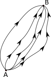
The path integral formulation is a description in quantum mechanics that generalizes the action principle of classical mechanics. It replaces the classical notion of a single, unique classical trajectory for a system with a sum, or functional integral, over an infinity of quantum-mechanically possible trajectories to compute a quantum amplitude.
In quantum mechanics and quantum field theory, the propagator is a function that specifies the probability amplitude for a particle to travel from one place to another in a given period of time, or to travel with a certain energy and momentum. In Feynman diagrams, which serve to calculate the rate of collisions in quantum field theory, virtual particles contribute their propagator to the rate of the scattering event described by the respective diagram. These may also be viewed as the inverse of the wave operator appropriate to the particle, and are, therefore, often called (causal) Green's functions.
In physics, the Hamilton–Jacobi equation, named after William Rowan Hamilton and Carl Gustav Jacob Jacobi, is an alternative formulation of classical mechanics, equivalent to other formulations such as Newton's laws of motion, Lagrangian mechanics and Hamiltonian mechanics. The Hamilton–Jacobi equation is particularly useful in identifying conserved quantities for mechanical systems, which may be possible even when the mechanical problem itself cannot be solved completely.
In mechanics, virtual work arises in the application of the principle of least action to the study of forces and movement of a mechanical system. The work of a force acting on a particle as it moves along a displacement is different for different displacements. Among all the possible displacements that a particle may follow, called virtual displacements, one will minimize the action. This displacement is therefore the displacement followed by the particle according to the principle of least action. The work of a force on a particle along a virtual displacement is known as the virtual work.
Electric potential energy, is a potential energy that results from conservative Coulomb forces and is associated with the configuration of a particular set of point charges within a defined system. An object may have electric potential energy by virtue of two key elements: its own electric charge and its relative position to other electrically charged objects.
In mathematics, in particular in algebraic geometry and differential geometry, Dolbeault cohomology is an analog of de Rham cohomology for complex manifolds. Let M be a complex manifold. Then the Dolbeault cohomology groups depend on a pair of integers p and q and are realized as a subquotient of the space of complex differential forms of degree (p,q).
The Frank–Tamm formula yields the amount of Cherenkov radiation emitted on a given frequency as a charged particle moves through a medium at superluminal velocity. It is named for Russian physicists Ilya Frank and Igor Tamm who developed the theory of the Cherenkov effect in 1937, for which they were awarded a Nobel Prize in Physics in 1958.
Defect types include atom vacancies, adatoms, steps, and kinks that occur most frequently at surfaces due to the finite material size causing crystal discontinuity. What all types of defects have in common, whether surface or bulk defects, is that they produce dangling bonds that have specific electron energy levels different from those of the bulk. This difference occurs because these states cannot be described with periodic Bloch waves due to the change in electron potential energy caused by the missing ion cores just outside the surface. Hence, these are localized states that require separate solutions to the Schrödinger equation so that electron energies can be properly described. The break in periodicity results in a decrease in conductivity due to defect scattering.
The electron-LA phonon interaction is an interaction that can take place between an electron and a longitudinal acoustic (LA) phonon in a material such as a semiconductor.
Multipole radiation is a theoretical framework for the description of electromagnetic or gravitational radiation from time-dependent distributions of distant sources. These tools are applied to physical phenomena which occur at a variety of length scales - from gravitational waves due to galaxy collisions to gamma radiation resulting from nuclear decay. Multipole radiation is analyzed using similar multipole expansion techniques that describe fields from static sources, however there are important differences in the details of the analysis because multipole radiation fields behave quite differently from static fields. This article is primarily concerned with electromagnetic multipole radiation, although the treatment of gravitational waves is similar.
In mathematics, the Neumann–Poincaré operator or Poincaré–Neumann operator, named after Carl Neumann and Henri Poincaré, is a non-self-adjoint compact operator introduced by Poincaré to solve boundary value problems for the Laplacian on bounded domains in Euclidean space. Within the language of potential theory it reduces the partial differential equation to an integral equation on the boundary to which the theory of Fredholm operators can be applied. The theory is particularly simple in two dimensions—the case treated in detail in this article—where it is related to complex function theory, the conjugate Beurling transform or complex Hilbert transform and the Fredholm eigenvalues of bounded planar domains.
Phase reduction is a method used to reduce a multi-dimensional dynamical equation describing a nonlinear limit cycle oscillator into a one-dimensional phase equation. Many phenomena in our world such as chemical reactions, electric circuits, mechanical vibrations, cardiac cells, and spiking neurons are examples of rhythmic phenomena, and can be considered as nonlinear limit cycle oscillators.