
In economics, profit maximization is the short run or long run process by which a firm may determine the price, input and output levels that will lead to the highest possible total profit. In neoclassical economics, which is currently the mainstream approach to microeconomics, the firm is assumed to be a "rational agent" which wants to maximize its total profit, which is the difference between its total revenue and its total cost.
Economies of scope are "efficiencies formed by variety, not volume". In economics, "economies" is synonymous with cost savings and "scope" is synonymous with broadening production/services through diversified products. Economies of scope is an economic theory stating that average total cost of production decrease as a result of increasing the number of different goods produced. For example, a gas station that sells gasoline can sell soda, milk, baked goods, etc. through their customer service representatives and thus gasoline companies achieve economies of scope.

The break-even point (BEP) in economics, business—and specifically cost accounting—is the point at which total cost and total revenue are equal, i.e. "even". There is no net loss or gain, and one has "broken even", though opportunity costs have been paid and capital has received the risk-adjusted, expected return. In short, all costs that must be paid are paid, and there is neither profit nor loss. The break-even analysis was developed by Karl Bücher and Johann Friedrich Schär.
In economics, the marginal cost is the change in the total cost that arises when the quantity produced is incremented, the cost of producing additional quantity. In some contexts, it refers to an increment of one unit of output, and in others it refers to the rate of change of total cost as output is increased by an infinitesimal amount. As Figure 1 shows, the marginal cost is measured in dollars per unit, whereas total cost is in dollars, and the marginal cost is the slope of the total cost, the rate at which it increases with output. Marginal cost is different from average cost, which is the total cost divided by the number of units produced.
A limit price is a price, or pricing strategy, where products are sold by a supplier at a price low enough to make it unprofitable for other players to enter the market.
Economic Order Quantity (EOQ), also known as Financial Purchase Quantity or Economic Buying Quantity (EPQ), is the order quantity that minimizes the total holding costs and ordering costs in inventory management. It is one of the oldest classical production scheduling models. The model was developed by Ford W. Harris in 1913, but R. H. Wilson, a consultant who applied it extensively, and K. Andler are given credit for their in-depth analysis.
Cournot competition is an economic model used to describe an industry structure in which companies compete on the amount of output they will produce, which they decide on independently of each other and at the same time. It is named after Antoine Augustin Cournot (1801–1877) who was inspired by observing competition in a spring water duopoly. It has the following features:
The Stackelberg leadership model is a strategic game in economics in which the leader firm moves first and then the follower firms move sequentially. It is named after the German economist Heinrich Freiherr von Stackelberg who published Marktform und Gleichgewicht [Market Structure and Equilibrium] in 1934, which described the model. In game theory terms, the players of this game are a leader and a follower and they compete on quantity. The Stackelberg leader is sometimes referred to as the Market Leader.
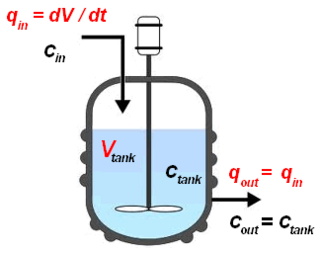
The continuous stirred-tank reactor (CSTR), also known as vat- or backmix reactor, mixed flow reactor (MFR), or a continuous-flow stirred-tank reactor (CFSTR), is a common model for a chemical reactor in chemical engineering and environmental engineering. A CSTR often refers to a model used to estimate the key unit operation variables when using a continuous agitated-tank reactor to reach a specified output. The mathematical model works for all fluids: liquids, gases, and slurries.
The economic lot scheduling problem (ELSP) is a problem in operations management and inventory theory that has been studied by many researchers for more than 50 years. The term was first used in 1958 by professor Jack D. Rogers of Berkeley, who extended the economic order quantity model to the case where there are several products to be produced on the same machine, so that one must decide both the lot size for each product and when each lot should be produced. The method illustrated by Jack D. Rogers draws on a 1956 paper from Welch, W. Evert. The ELSP is a mathematical model of a common issue for almost any company or industry: planning what to manufacture, when to manufacture and how much to manufacture.
The newsvendormodel is a mathematical model in operations management and applied economics used to determine optimal inventory levels. It is (typically) characterized by fixed prices and uncertain demand for a perishable product. If the inventory level is , each unit of demand above is lost in potential sales. This model is also known as the newsvendor problem or newsboy problem by analogy with the situation faced by a newspaper vendor who must decide how many copies of the day's paper to stock in the face of uncertain demand and knowing that unsold copies will be worthless at the end of the day.
The economic production quantity model determines the quantity a company or retailer should order to minimize the total inventory costs by balancing the inventory holding cost and average fixed ordering cost. The EPQ model was developed by E.W. Taft in 1918. This method is an extension of the economic order quantity model. The difference between these two methods is that the EPQ model assumes the company will produce its own quantity or the parts are going to be shipped to the company while they are being produced, therefore the orders are available or received in an incremental manner while the products are being produced. While the EOQ model assumes the order quantity arrives complete and immediately after ordering, meaning that the parts are produced by another company and are ready to be shipped when the order is placed.
Field inventory management, commonly known as inventory management is the function of understanding the stock mix of a company and the different demands on that stock. The demands are influenced by both external and internal factors and are balanced by the creation of purchase order requests to keep supplies at a reasonable or prescribed level. Inventory management is important for every other business enterprise.
Material theory is the sub-specialty within operations research and operations management that is concerned with the design of production/inventory systems to minimize costs: it studies the decisions faced by firms and the military in connection with manufacturing, warehousing, supply chains, spare part allocation and so on and provides the mathematical foundation for logistics. The inventory control problem is the problem faced by a firm that must decide how much to order in each time period to meet demand for its products. The problem can be modeled using mathematical techniques of optimal control, dynamic programming and network optimization. The study of such models is part of inventory theory.
The dynamic lot-size model in inventory theory, is a generalization of the economic order quantity model that takes into account that demand for the product varies over time. The model was introduced by Harvey M. Wagner and Thomson M. Whitin in 1958.
The Silver–Meal heuristic is a production planning method in manufacturing, composed in 1973 by Edward A. Silver and H.C. Meal. Its purpose is to determine production quantities to meet the requirement of operations at minimum cost.
The profit model is the linear, deterministic algebraic model used implicitly by most cost accountants. Starting with, profit equals sales minus costs, it provides a structure for modeling cost elements such as materials, losses, multi-products, learning, depreciation etc. It provides a mutable conceptual base for spreadsheet modelers. This enables them to run deterministic simulations or 'what if' modelling to see the impact of price, cost or quantity changes on profitability.

In microeconomics, a monopoly price is set by a monopoly. A monopoly occurs when a firm lacks any viable competition and is the sole producer of the industry's product. Because a monopoly faces no competition, it has absolute market power and can set a price above the firm's marginal cost.
The base stock model is a statistical model in inventory theory. In this model inventory is refilled one unit at a time and demand is random. If there is only one replenishment, then the problem can be solved with the newsvendor model.
The (Q,r) model is a class of models in inventory theory. A general (Q,r) model can be extended from both the EOQ model and the base stock model


