Flood fill

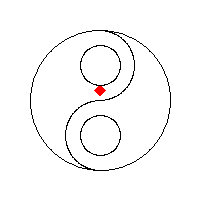
Recursive flood fill with 4 directions

Flood fill, also called seed fill, is a flooding algorithm that determines and alters the area connected to a given node in a multi-dimensional array with some matching attribute. It is used in the "bucket" fill tool of paint programs to fill connected, similarly colored areas with a different color, and in games such as Go and Minesweeper for determining which pieces are cleared. A variant called boundary fill uses the same algorithms but is defined as the area connected to a given node that does not have a particular attribute. ^[1]

Note that flood filling is not suitable for drawing filled polygons, as it will miss some pixels in more acute corners. ^[2] Instead, see Even-odd rule and Nonzero-rule.

The algorithm parameters

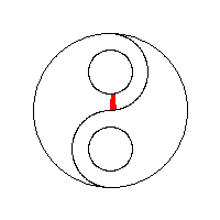
Recursive flood fill with 8 directions

The traditional flood-fill algorithm takes three parameters: a start node, a target color, and a replacement color. The algorithm looks for all nodes in the array that are connected to the start node by a path of the target color and changes them to the replacement color. For a boundary-fill, in place of the target color, a border color would be supplied.

In order to generalize the algorithm in the common way, the following descriptions will instead have two routines available. ^[3] One called Inside which returns true for unfilled points that, by their color, would be inside the filled area, and one called Set which fills a pixel/node. Any node that has Set called on it must then no longer be Inside.

Depending on whether we consider nodes touching at the corners connected or not, we have two variations: eight-way and four-way respectively.

Stack-based recursive implementation (four-way)

The earliest-known, implicitly stack-based, recursive, four-way flood-fill implementation goes as follows: ^{[4] [5] [6] [7]}

Flood-fill (node):  1. If node is not Inside return.  2. Set the node  3. Perform Flood-fill one step to the south of node.  4. Perform Flood-fill one step to the north of node  5. Perform Flood-fill one step to the west of node  6. Perform Flood-fill one step to the east of node  7. Return.

Though easy to understand, the implementation of the algorithm used above is impractical in languages and environments where stack space is severely constrained (e.g. Microcontrollers).

Moving the recursion into a data structure

Four-way flood fill using a queue for storage

Four-way flood fill using a stack for storage

Moving the recursion into a data structure (either a stack or a queue) prevents a stack overflow. It is similar to the simple recursive solution, except that instead of making recursive calls, it pushes the nodes onto a stack or queue for consumption, with the choice of data structure affecting the proliferation pattern:

Flood-fill (node):   1. Set Q to the empty queue or stack.   2. Add node to the end of Q.   3. While Q is not empty:   4.   Set n equal to the first element of Q.   5.   Remove first element from Q.   6.   If n is Inside:          Set the n          Add the node to the west of n to the end of Q.          Add the node to the east of n to the end of Q.          Add the node to the north of n to the end of Q.          Add the node to the south of n to the end of Q.   7. Continue looping until Q is exhausted.   8. Return.

Further potential optimizations

• Check and set each node's pixel color before adding it to the stack/queue, reducing stack/queue size.
• Use a loop for the east–west directions, queuing pixels above/below as you go (making it similar to the span filling algorithms, below).
• Interleave two or more copies of the code with extra stacks/queues, to allow out-of-order processors more opportunity to parallelize.
• Use multiple threads (ideally with slightly different visiting orders, so they don't stay in the same area). ^[6]

Advantages

• Very simple algorithm - easy to make bug-free. ^[6]

Disadvantages

• Uses a lot of memory, particularly when using a stack. ^[6]
• Tests most filled pixels a total of four times.
• Not suitable for pattern filling, as it requires pixel test results to change.
• Access pattern is not cache-friendly, for the queuing variant.
• Cannot easily optimize for multi-pixel words or bitplanes. ^[2]

Span filling

Scanline fill using a stack for storage

It's possible to optimize things further by working primarily with spans, a row with constant y. The first published complete example works on the following basic principle. ^[1]

1. Starting with a seed point, fill left and right. Keep track of the leftmost filled point lx and rightmost filled point rx. This defines the span.
2. Scan from lx to rx above and below the seed point, searching for new seed points to continue with.

As an optimisation, the scan algorithm does not need restart from every seed point, but only those at the start of the next span. Using a stack explores spans depth first, whilst a queue explores spans breadth first.

fn fill(x, y):     if not Inside(x, y) then return     let s = new empty stack or queue     Add (x, y) to s     while s is not empty:         Remove an (x, y) from s         let lx = x         while Inside(lx - 1, y):             Set(lx - 1, y)             lx = lx - 1         while Inside(x, y):             Set(x, y)             x = x + 1       scan(lx, x - 1, y + 1, s)       scan(lx, x - 1, y - 1, s)  fn scan(lx, rx, y, s):     let span_added = false     for x in lx .. rx:         if not Inside(x, y):             span_added = false         else if not span_added:             Add (x, y) to sspan_added = true

Over time, the following optimizations were realized:

• When a new scan would be entirely within a grandparent span, it would certainly only find filled pixels, and so wouldn't need queueing. ^{[1] [6] [3]}
• Further, when a new scan overlaps a grandparent span, only the overhangs (U-turns and W-turns) need to be scanned. ^[3]
• It's possible to fill while scanning for seeds ^[6]

The final, combined-scan-and-fill span filler was then published in 1990. In pseudo-code form: ^[8]

fn fill(x, y):     if not Inside(x, y) then return     let s = new empty queue or stack     Add (x, x, y, 1) to s     Add (x, x, y - 1, -1) to s     while s is not empty:         Remove an (x1, x2, y, dy) from s         let x = x1         if Inside(x, y):             while Inside(x - 1, y):                 Set(x - 1, y)                 x = x - 1             if x < x1:                 Add (x, x1 - 1, y - dy, -dy) to s         while x1 <= x2:             while Inside(x1, y):                 Set(x1, y)                 x1 = x1 + 1             if x1 > x:                 Add (x, x1 - 1, y + dy, dy) to s             if x1 - 1 > x2:                 Add (x2 + 1, x1 - 1, y - dy, -dy) to sx1 = x1 + 1             while x1 < x2 and not Inside(x1, y):                 x1 = x1 + 1             x = x1

Advantages

• 2–8x faster than the pixel-recursive algorithm.
• Access pattern is cache and bitplane-friendly. ^[6]
• Can draw a horizontal line rather than setting individual pixels. ^[6]

Disadvantages

• Still visits pixels it has already filled. (For the popular algorithm, 3 scans of most pixels. For the final one, only doing extra scans of pixels where there are holes in the filled area.) ^[3]
• Not suitable for pattern filling, as it requires pixel test results to change.

Adding pattern filling support

Two common ways to make the span and pixel-based algorithms support pattern filling are either to use a unique color as a plain fill and then replace that with a pattern or to keep track (in a 2d boolean array or as regions) of which pixels have been visited, using it to indicate pixels are no longer fillable. Inside must then return false for such visited pixels. ^[3]

Graph-theoretic filling

Some theorists applied explicit graph theory to the problem, treating spans of pixels, or aggregates of such, as nodes and studying their connectivity. The first published graph theory algorithm worked similarly to the span filling, above, but had a way to detect when it would duplicate filling of spans. ^[9] Unfortunately, it had bugs that made it not complete some fills. ^[10] A corrected algorithm was later published with a similar basis in graph theory; however, it alters the image as it goes along, to temporarily block off potential loops, complicating the programmatic interface. ^[10] A later published algorithm depended on the boundary being distinct from everything else in the image and so isn't suitable for most uses; ^{[11] [3]} it also requires an extra bit per pixel for bookkeeping. ^[3]

Advantages

• Suitable for pattern filling, directly, as it never retests filled pixels. ^{[9] [10] [11]}
• Double the speed of the original span algorithm, for uncomplicated fills. ^[3]
• Access pattern is cache and bitplane-friendly. ^{[6] [3]}

Disadvantages

• Regularly, a span has to be compared to every other 'front' in the queue, which significantly slows down complicated fills. ^[3]
• Switching back and forth between graph theoretic and pixel domains complicates understanding.
• The code is fairly complicated, increasing the chances of bugs.

Walk-based filling (Fixed-memory method)

A method exists that uses essentially no memory for four-connected regions by pretending to be a painter trying to paint the region without painting themselves into a corner. This is also a method for solving mazes. The four pixels making the primary boundary are examined to see what action should be taken. The painter could find themselves in one of several conditions:

1. All four boundary pixels are filled.
2. Three of the boundary pixels are filled.
3. Two of the boundary pixels are filled.
4. One boundary pixel is filled.
5. Zero boundary pixels are filled.

Where a path or boundary is to be followed, the right-hand rule is used. The painter follows the region by placing their right-hand on the wall (the boundary of the region) and progressing around the edge of the region without removing their hand.

For case #1, the painter paints (fills) the pixel the painter is standing upon and stops the algorithm.

For case #2, a path leading out of the area exists. Paint the pixel the painter is standing upon and move in the direction of the open path.

For case #3, the two boundary pixels define a path which, if we painted the current pixel, may block us from ever getting back to the other side of the path. We need a "mark" to define where we are and which direction we are heading to see if we ever get back to exactly the same pixel. If we already created such a "mark", then we preserve our previous mark and move to the next pixel following the right-hand rule.

A mark is used for the first 2-pixel boundary that is encountered to remember where the passage started and in what direction the painter was moving. If the mark is encountered again and the painter is traveling in the same direction, then the painter knows that it is safe to paint the square with the mark and to continue in the same direction. This is because (through some unknown path) the pixels on the other side of the mark can be reached and painted in the future. The mark is removed for future use.

If the painter encounters the mark but is going in a different direction, then some sort of loop has occurred, which caused the painter to return to the mark. This loop must be eliminated. The mark is picked up, and the painter then proceeds in the direction indicated previously by the mark using a left-hand rule for the boundary (similar to the right-hand rule but using the painter's left hand). This continues until an intersection is found (with three or more open boundary pixels). Still using the left-hand rule the painter now searches for a simple passage (made by two boundary pixels). Upon finding this two-pixel boundary path, that pixel is painted. This breaks the loop and allows the algorithm to continue.

For case #4, we need to check the opposite 8-connected corners to see whether they are filled or not. If either or both are filled, then this creates a many-path intersection and cannot be filled. If both are empty, then the current pixel can be painted and the painter can move following the right-hand rule.

The algorithm trades time for memory. For simple shapes it is very efficient. However, if the shape is complex with many features, the algorithm spends a large amount of time tracing the edges of the region trying to ensure that all can be painted.

A walking algorithm was published in 1994. ^[12]

Pseudocode

This is a pseudocode implementation of an optimal fixed-memory flood-fill algorithm written in structured English:

The variables

• cur, mark, and mark2 each hold either pixel coordinates or a null value
  • NOTE: when mark is set to null, do not erase its previous coordinate value. Keep those coordinates available to be recalled if necessary.
• cur-dir, mark-dir, and mark2-dir each hold a direction (left, right, up, or down)
• backtrack and findloop each hold boolean values
• count is an integer

The algorithm

NOTE: All directions (front, back, left, right) are relative to cur-dir

set cur to starting pixel set cur-dir to default direction clear mark and mark2 (set values to null) set backtrack and findloop to false  while front-pixel is empty do     move forward end while  jump to START  MAIN LOOP:     move forward     if right-pixel is inside thenif backtrack is true and findloop is false and either front-pixel or left-pixel is inside then             set findloop to true         end if         turn right PAINT:         move forward     end if START:     setcount to number of non-diagonally adjacent pixels filled (front/back/left/right ONLY)     ifcountis not 4 thendo             turn right         while front-pixel is inside         do             turn left         while front-pixel is not inside     end ifswitchcount         case 1             if backtrack is true then                 set findloop to true             else if findloop is true thenif mark is null then                     restore mark                 end ifelse if front-left-pixel and back-left-pixel are both inside then                 clear mark                 set cur                 jump to PAINT             end if         end case         case 2             if back-pixel is not inside thenif front-left-pixel is inside then                     clear mark                     set cur                     jump to PAINT                 end ifelse if mark is not set then                 set mark to cur                 set mark-dir to cur-dir                 clear mark2                 set findloop and backtrack to false             elseif mark2 is not set thenif cur is at mark thenif cur-dir is the same as mark-dir then                             clear mark                             turn around                             set cur                             jump to PAINT                         else                             set backtrack to true                             set findloop to false                             set cur-dir to mark-dir                         end ifelse if findloop is true then                         set mark2 to cur                         set mark2-dir to cur-dir                     end ifelseif cur is at mark then                         set cur to mark2                         set cur-dir to mark2-dir                         clear mark and mark2                         set backtrack to false                         turn around                         set cur                         jump to PAINT                     else if cur at mark2 then                         set mark to cur                         set cur-dir and mark-dir to mark2-dir                         clear mark2                     end ifend ifend if         end case         case 3             clear mark             set cur             jump to PAINT         end case         case 4             set cur             done         end case     end switch end MAIN LOOP

Advantages

• Constant memory usage.

Disadvantages

• Access pattern is not cache or bitplane-friendly.
• Can spend a lot of time walking around loops before closing them.

Vector implementations

Version 0.46 of Inkscape includes a bucket fill tool, giving output similar to ordinary bitmap operations and indeed using one: the canvas is rendered, a flood fill operation is performed on the selected area and the result is then traced back to a path. It uses the concept of a boundary condition.

See also

• Breadth-first search
• Depth-first search
• Graph traversal
• Connected-component labeling
• Dijkstra's algorithm
• Watershed (image processing)

External links

• Sample implementations for recursive and non-recursive, classic and scanline flood fill, by Lode Vandevenne.
• Sample Java implementation using Q non-recursive.

References

1. Smith, Alvy Ray (1979). Tint Fill. SIGGRAPH '79: Proceedings of the 6th annual conference on Computer graphics and interactive techniques. pp. 276–283. doi:10.1145/800249.807456.
2. Ackland, Bryan D; Weste, Neil H (1981). The edge flag algorithm — A fill method for raster scan displays. IEEE Transactions on Computers (Volume: C-30, Issue: 1). pp. 41–48. doi:10.1109/TC.1981.6312155.
3. Fishkin, Kenneth P; Barsky, Brian A (1985). An Analysis and Algorithm for Filling Propagation. Computer-Generated Images: The State of the Art Proceedings of Graphics Interface ’85. pp. 56–76. doi:10.1007/978-4-431-68033-8_6.
4. Newman, William M; Sproull, Robert Fletcher (1979). Principles of Interactive Computer Graphics (2nd ed.). McGraw-Hill. p. 253. ISBN   978-0-07-046338-7.
5. Pavlidis, Theo (1982). Algorithms for Graphics and Image Processing. Springer-Verlag. p. 181. ISBN   978-3-642-93210-6.
6. Levoy, Marc (1982). Area Flooding Algorithms. SIGGRAPH 1981 Two-Dimensional Computer Animation course notes.
7. Foley, J D; van Dam, A; Feiner, S K; Hughes, S K (1990). Computer Graphics: Principles and Practice (2nd ed.). Addison–Wesley. pp. 979–982. ISBN   978-0-201-84840-3.
8. Heckbert, Paul S (1990). "IV.10: A Seed Fill Algorithm". In Glassner, Andrew S (ed.). Graphics Gems. Academic Press. pp. 275–277. ISBN   0122861663.
9. Lieberman, Henry (1978). How to Color in a Coloring Book. SIGGRAPH '78: Proceedings of the 5th annual conference on Computer graphics and interactive techniques. pp. 111–116. doi:10.1145/800248.807380.
10. Shani, Uri (1980). Filling regions in binary raster images: A graph-theoretic approach. SIGGRAPH '80: Proceedings of the 7th annual conference on Computer graphics and interactive techniques. pp. 321–327. doi:10.1145/800250.807511.
11. Pavlidis, Theo (1981). Contour Filling in Raster Graphics. SIGGRAPH '81: Proceedings of the 8th annual conference on Computer graphics and interactive techniques. pp. 29–36. doi:10.1145/800224.806786.
12. Henrich, Dominik (1994). Space-efficient region filling in raster graphics. The Visual Computer. pp. 205–215. doi:10.1007/BF01901287.