Animated example of a breadth-first search. Black: explored, grey: queued to be explored later onBFS on Maze-solving algorithmTop part of Tic-tac-toe game tree
Breadth-first search (BFS) is an algorithm for searching a tree data structure for a node that satisfies a given property. It starts at the tree root and explores all nodes at the present depth prior to moving on to the nodes at the next depth level. Extra memory, usually a queue, is needed to keep track of the child nodes that were encountered but not yet explored.
For example, in a chess endgame, a chess engine may build the game tree from the current position by applying all possible moves and use breadth-first search to find a winning position for White. Implicit trees (such as game trees or other problem-solving trees) may be of infinite size; breadth-first search is guaranteed to find a solution node[1] if one exists.
In contrast, (plain) depth-first search (DFS), which explores the node branch as far as possible before backtracking and expanding other nodes,[2] may get lost in an infinite branch and never make it to the solution node. Iterative deepening depth-first search avoids the latter drawback at the price of exploring the tree's top parts over and over again. On the other hand, both depth-first algorithms typically require far less extra memory than breadth-first search.[3]
Breadth-first search can be generalized to both undirected graphs and directed graphs with a given start node (sometimes referred to as a 'search key').[4] In state space search in artificial intelligence, repeated searches of vertices are often allowed, while in theoretical analysis of algorithms based on breadth-first search, precautions are typically taken to prevent repetitions.
BFS and its application in finding connected components of graphs were invented in 1945 by Konrad Zuse, in his (rejected) Ph.D. thesis on the Plankalkül programming language, but this was not published until 1972.[5] It was reinvented in 1959 by Edward F. Moore, who used it to find the shortest path out of a maze,[6][7] and later developed by C. Y. Lee into a wire routing algorithm (published in 1961).[8]
Pseudocode
Input: A graph G and a starting vertex root of G
Output: Goal state. The parent links trace the shortest path back to root[9]
1 procedure BFS(G, root) is 2 let Q be a queue 3 label root as explored 4 Q.enqueue(root) 5 whileQ is not empty do 6 v := Q.dequeue() 7 ifv is the goal then 8 returnv 9 for all edges from v to winG.adjacentEdges(v) do 10 ifw is not labeled as explored then 11 label w as explored 12 w.parent := v 13 Q.enqueue(w)
More details
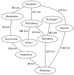
An example map of Southern Germany with some connections between citiesThe breadth-first tree obtained when running BFS on the given map and starting in Frankfurt
This non-recursive implementation is similar to the non-recursive implementation of depth-first search, but differs from it in two ways:
it checks whether a vertex has been explored before enqueueing the vertex rather than delaying this check until the vertex is dequeued from the queue.
If G is a tree, replacing the queue of this breadth-first search algorithm with a stack will yield a depth-first search algorithm. For general graphs, replacing the stack of the iterative depth-first search implementation with a queue would also produce a breadth-first search algorithm, although a somewhat nonstandard one.[10]
The Q queue contains the frontier along which the algorithm is currently searching.
Nodes can be labelled as explored by storing them in a set, or by an attribute on each node, depending on the implementation.
Note that the word node is usually interchangeable with the word vertex.
The parent attribute of each node is useful for accessing the nodes in a shortest path, for example by backtracking from the destination node up to the starting node, once the BFS has been run, and the predecessors nodes have been set.
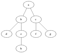
Breadth-first search produces a breadth-first tree which is shown in the example below.
Example
The lower diagram shows the breadth-first tree obtained by running a BFS on an example graph of German cities (upper diagram) starting from Frankfurt.
Analysis
Time and space complexity
The time complexity can be expressed as , as every vertex and every edge will be explored in the worst case. is the number of vertices and is the number of edges in the graph. Note that may vary between and , depending on how sparse the input graph is.[11]
When the number of vertices in the graph is known ahead of time, and additional data structures are used to determine which vertices have already been added to the queue, the space complexity can be expressed as , where is the number of vertices. This is in addition to the space required for the graph itself, which may vary depending on the graph representation used by an implementation of the algorithm.
When working with graphs that are too large to store explicitly (or infinite), it is more practical to describe the complexity of breadth-first search in different terms: to find the nodes that are at distance d from the start node (measured in number of edge traversals), BFS takes O(bd + 1) time and memory, where b is the "branching factor" of the graph (the average out-degree).[12]:81
Completeness
In the analysis of algorithms, the input to breadth-first search is assumed to be a finite graph, represented as an adjacency list, adjacency matrix, or similar representation. However, in the application of graph traversal methods in artificial intelligence the input may be an implicit representation of an infinite graph. In this context, a search method is described as being complete if it is guaranteed to find a goal state if one exists. Breadth-first search is complete, but depth-first search is not. When applied to infinite graphs represented implicitly, breadth-first search will eventually find the goal state, but depth first search may get lost in parts of the graph that have no goal state and never return.[13]
BFS ordering
An enumeration of the vertices of a graph is said to be a BFS ordering if it is a possible output of the application of BFS to this graph.
Let be a graph with vertices. Recall that is the set of neighbors of . Let be a list of distinct elements of , for , let be the least such that is a neighbor of , if such a exists, and be otherwise.
Let be an enumeration of the vertices of . The enumeration is said to be a BFS ordering (with source ) if, for all , is the vertex such that is minimal. Equivalently, is a BFS ordering if, for all with , there exists a neighbor of such that .
Applications
Breadth-first search can be used to solve many problems in graph theory, for example:
↑ Zuse, Konrad (1972), Der Plankalkül (in German), Konrad Zuse Internet Archive. See pp. 96–105 of the linked pdf file (internal numbering 2.47–2.56).
↑ Moore, Edward F. (1959). "The shortest path through a maze". Proceedings of the International Symposium on the Theory of Switching. Harvard University Press. pp.285–292. As cited by Cormen, Leiserson, Rivest, and Stein.
↑ Lee, C. Y. (1961). "An Algorithm for Path Connections and Its Applications". IRE Transactions on Electronic Computers (3): 346–365. doi:10.1109/TEC.1961.5219222. S2CID40700386.
This page is based on this Wikipedia article Text is available under the CC BY-SA 4.0 license; additional terms may apply. Images, videos and audio are available under their respective licenses.