Group method of data handling (GMDH) is a family of inductive, self-organizing algorithms for mathematical modelling that automatically determines the structure and parameters of models based on empirical data. GMDH iteratively generates and evaluates candidate models, often using polynomial functions, and selects the best-performing ones based on an external criterion. This process builds feedforward networks of optimal complexity, adapting to the noise level in the data and minimising overfitting, ensuring that the resulting model is accurate and generalizable.[1]
GMDH is used in such fields as machine learning, forecasting, optimization and pattern recognition, due to its ability to handle complex, nonlinear relationships in data. Its inductive nature allows it to discover patterns and interdependencies without requiring strong a priori assumptions, making it particularly effective for highly complex systems. By balancing model complexity and accuracy through self-organization, GMDH ensures that the model reflects the underlying relationships in data.[2] This approach has influenced modern machine learning techniques and is recognised as one of the earliest approaches to automated machine learning and deep learning.
A GMDH model with multiple inputs and one output is a subset of components of the base function (1):
where fi are elementary functions dependent on different sets of inputs, ai are coefficients and m is the number of the base function components.
In order to find the best solution, GMDH algorithms consider various component subsets of the base function (1) called partial models. Coefficients of these models are estimated by the least squares method. GMDH algorithms gradually increase the number of partial model components and find a model structure with optimal complexity indicated by the minimum value of an external criterion. This process is called self-organization of models.
Usually, more simple partial models with up to second degree functions are used.[1]
Other names include "heuristic self-organization of models" or "polynomial feedforward neural network".[3]Jürgen Schmidhuber cites GMDH as one of the first deep learning methods, remarking that it was used to train eight-layer neural nets as early as 1971.[4][5]
History
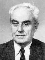
GMDH author – Soviet and Ukrainian scientist Prof. Alexey G. Ivakhnenko
The method was originated in 1968 by Prof. Alexey G. Ivakhnenko at the Institute of Cybernetics in Kyiv. This inductive approach from the very beginning was a computer-based method, so a set of computer programs and algorithms were the primary practical results achieved at the base of the new theoretical principles. Thanks to the author's policy of open code sharing, the method was quickly settled in the large number of scientific laboratories worldwide. As most routine work is transferred to a computer, the impact of human influence on the objective result is minimised. In fact, this approach can be considered as one of the implementations of the Artificial Intelligence thesis, which states that a computer can act as a powerful advisor to humans.
The development of GMDH consists of a synthesis of ideas from different areas of science: the cybernetic concept of "black box"[6] and the principle of successive genetic selection of pairwise features, Godel's incompleteness theorems and the Gabor's principle of "freedom of decisions choice",[7] and the Beer's principle of external additions.[8]
GMDH is the original method for solving problems for structural-parametric identification of models for experimental data under uncertainty.[9] Such a problem occurs in the construction of a mathematical model that approximates the unknown pattern of investigated object or process.[10] It uses information about it that is implicitly contained in data. GMDH differs from other methods of modelling by the active application of the following principles: automatic models generation, inconclusive decisions, and consistent selection by external criteria for finding models of optimal complexity. It had an original multilayered procedure for automatic models structure generation, which imitates the process of biological selection with consideration of pairwise successive features. Such procedure is currently used in deep learning networks.[11] To compare and choose optimal models, two or more subsets of a data sample are used. This makes it possible to avoid preliminary assumptions because sample division implicitly acknowledges different types of uncertainty during the automatic construction of the optimal model.
During development was established an organic analogy between the problem of constructing models for noisy data and signal passing through the channel with noise.[12] This made possible to lay the foundations of the theory of noise-immune modelling.[9] The main result of this theory is that the complexity of optimal predictive model depends on the level of uncertainty in the data: the higher this level (e.g. due to noise) - the simpler must be the optimal model (with less estimated parameters). This initiated the development of the GMDH theory as an inductive method of automatic adaptation of optimal model complexity to the level of noise variation in fuzzy data. Therefore, GMDH is often considered to be the original information technology for knowledge extraction from experimental data.
Period 1968–1971 is characterized by the application of only regularity criterion for solving of the problems of identification, pattern recognition and short-term forecasting. As reference functions, polynomials, logical nets, fuzzy Zadeh sets and Bayes probability formulas were used. Authors were stimulated by the very high accuracy of forecasting with the new approach. Noise immunity was not investigated.
Period 1972–1975. The problem of modeling of noised data and incomplete information basis was solved. Multicriteria selection and the utilisation of additional a priori information for noise immunity increase were proposed. The best experiments showed that, with an extended definition of the optimal model by an additional criterion, the noise level can be ten times greater than the signal. Then it was improved using Shannon's Theorem of General Communication theory.
Period 1976–1979. The convergence of multilayered GMDH algorithms was investigated. It has been demonstrated that some multilayered algorithms exhibit a form of error analogous to the static error of control systems, known as 'multilayerness error'. In 1977, a solution of objective systems analysis problems by multilayered GMDH algorithms was proposed. It turned out that sorting-out by criteria ensemble finds the only optimal system of equations and therefore to show complex object elements, their main input and output variables.
Period 1980–1988. Many important theoretical results were received. It became clear that full physical models cannot be used for long-term forecasting. It was proved, that non-physical models of GMDH are more accurate for approximation and forecast than physical models of regression analysis. Two-level algorithms which use two different time scales for modeling were developed.
Since 1989 the new algorithms (AC, OCC, PF) for non-parametric modeling of fuzzy objects and SLP for expert systems were developed and investigated.[13] The present stage of GMDH development can be described as a blossoming of deep learning neural networks and parallel inductive algorithms for multiprocessor computers.
External criteria
External criterion is one of the key features of GMDH. This criterion describes requirements to the model, for example minimization of Least squares. It is always calculated with a separate part of data sample that has not been used for estimation of coefficients. This makes it possible to select a model of optimal complexity according to the level of uncertainty in input data. There are several popular criteria:
Criterion of Regularity (CR) – Least squares of a model at the sample B.
Criterion of Minimum bias or Consistency – a squared error of difference between the estimated outputs (or coefficients vectors) of two models developed on the basis of two distinct samples A and B, divided by squared output estimated on sample B. Comparison of models using it, enables to get consistent models and recover a hidden physical law from the noisy data.[1]
A simple description of model development using GMDH
For modeling using GMDH, only the selection criterion and maximum model complexity are pre-selected. Then, the design process begins from the first layer and goes on. The number of layers and neurons in hidden layers, model structure are determined automatically. All possible combinations of allowable inputs (all possible neurons) can be considered. Then polynomial coefficients are determined using one of the available minimizing methods such as singular value decomposition (with training data). Then, neurons that have better external criterion value (for testing data) are kept, and others are removed. If the external criterion for layer's best neuron reach minimum or surpasses the stopping criterion, network design is completed and the polynomial expression of the best neuron of the last layer is introduced as the mathematical prediction function; if not, the next layer will be generated, and this process goes on.[14]
GMDH-type neural networks
There are many different ways to choose an order for partial models consideration. The very first consideration order used in GMDH and originally called multilayered inductive procedure is the most popular one. It is a sorting-out of gradually complicated models generated from base function. The best model is indicated by the minimum of the external criterion characteristic. The multilayered procedure is equivalent to the Artificial Neural Network with polynomial activation function of neurons. Therefore, the algorithm with such an approach usually referred as GMDH-type Neural Network or Polynomial Neural Network. Li showed that GMDH-type neural network performed better than the classical forecasting algorithms such as Single Exponential Smooth, Double Exponential Smooth, ARIMA and back-propagation neural network.[15]
Combinatorial GMDH
Fig.1. A typical distribution of minimal values of criterion of regularity for Combinatorial GMDH models with different complexity.
Another important approach to partial models consideration that is becoming more and more popular is a combinatorial search that is either limited or full. This approach has some advantages against Polynomial Neural Networks, but requires considerable computational power and thus is not effective for objects with a large number of inputs. An important achievement of Combinatorial GMDH is that it fully outperforms linear regression approach if the noise level in the input data is greater than zero. It guarantees that the most optimal model will be founded during exhaustive sorting.
Basic Combinatorial algorithm makes the following steps:
Divides data sample at least into two samples A and B.
Generates subsamples from A according to partial models with steadily increasing complexity.
Estimates coefficients of partial models at each layer of models complexity.
Calculates value of external criterion for models on sample B.
Chooses the best model (set of models) indicated by minimal value of the criterion.
For the selected model of optimal complexity recalculate coefficients on a whole data sample.
In contrast to GMDH-type neural networks, the Combinatorial algorithm usually does not stop at the certain level of complexity because a point of increase in criterion value can be simply a local minimum, see Fig.1.
Algorithms
Combinatorial (COMBI)
Multilayered Iterative (MIA)
GN
Objective System Analysis (OSA)
Harmonical
Two-level (ARIMAD)
Multiplicative–Additive (MAA)
Objective Computer Clusterization (OCC);
Pointing Finger (PF) clusterization algorithm;
Analogues Complexing (AC)
Harmonical Re-discretization
Algorithm on the base of Multilayered Theory of Statistical Decisions (MTSD)
GEvom — Free upon request for academic use. Windows-only.
GMDH Shell — GMDH-based, predictive analytics and time series forecasting software. Free Academic Licensing and Free Trial version available. Windows-only.
KnowledgeMiner — Commercial product. Mac OS X-only. Free Demo version available.
↑Ivakhnenko, O.G.; Lapa, V.G. (1967). Cybernetics and Forecasting Techniques (Modern Analytic and Computational Methods in Science and Mathematics, v.8ed.). American Elsevier.
↑Takao, S.; Kondo, S.; Ueno, J.; Kondo, T. (2017). "Deep feedback GMDH-type neural network and its application to medical image analysis of MRI brain images". Artificial Life and Robotics. 23 (2): 161–172. doi:10.1007/s10015-017-0410-1. S2CID44190434.
↑Sohani, Ali; Sayyaadi, Hoseyn; Hoseinpoori, Sina (2016-09-01). "Modeling and multi-objective optimization of an M-cycle cross-flow indirect evaporative cooler using the GMDH type neural network". International Journal of Refrigeration. 69: 186–204. doi:10.1016/j.ijrefrig.2016.05.011.
↑Li, Rita Yi Man; Fong, Simon; Chong, Kyle Weng Sang (2017). "Forecasting the REITs and stock indices: Group Method of Data Handling Neural Network approach". Pacific Rim Property Research Journal. 23 (2): 123–160. doi:10.1080/14445921.2016.1225149. S2CID157150897.
This page is based on this Wikipedia article Text is available under the CC BY-SA 4.0 license; additional terms may apply. Images, videos and audio are available under their respective licenses.