
Protein secondary structure is the local spatial conformation of the polypeptide backbone excluding the side chains. The two most common secondary structural elements are alpha helices and beta sheets, though beta turns and omega loops occur as well. Secondary structure elements typically spontaneously form as an intermediate before the protein folds into its three dimensional tertiary structure.

Protein structure prediction is the inference of the three-dimensional structure of a protein from its amino acid sequence—that is, the prediction of its secondary and tertiary structure from primary structure. Structure prediction is different from the inverse problem of protein design. Protein structure prediction is one of the most important goals pursued by computational biology; and it is important in medicine and biotechnology.

Structural alignment attempts to establish homology between two or more polymer structures based on their shape and three-dimensional conformation. This process is usually applied to protein tertiary structures but can also be used for large RNA molecules. In contrast to simple structural superposition, where at least some equivalent residues of the two structures are known, structural alignment requires no a priori knowledge of equivalent positions. Structural alignment is a valuable tool for the comparison of proteins with low sequence similarity, where evolutionary relationships between proteins cannot be easily detected by standard sequence alignment techniques. Structural alignment can therefore be used to imply evolutionary relationships between proteins that share very little common sequence. However, caution should be used in using the results as evidence for shared evolutionary ancestry because of the possible confounding effects of convergent evolution by which multiple unrelated amino acid sequences converge on a common tertiary structure.

Structural bioinformatics is the branch of bioinformatics that is related to the analysis and prediction of the three-dimensional structure of biological macromolecules such as proteins, RNA, and DNA. It deals with generalizations about macromolecular 3D structures such as comparisons of overall folds and local motifs, principles of molecular folding, evolution, binding interactions, and structure/function relationships, working both from experimentally solved structures and from computational models. The term structural has the same meaning as in structural biology, and structural bioinformatics can be seen as a part of computational structural biology. The main objective of structural bioinformatics is the creation of new methods of analysing and manipulating biological macromolecular data in order to solve problems in biology and generate new knowledge.
An epitope, also known as antigenic determinant, is the part of an antigen that is recognized by the immune system, specifically by antibodies, B cells, or T cells. The part of an antibody that binds to the epitope is called a paratope. Although epitopes are usually non-self proteins, sequences derived from the host that can be recognized are also epitopes.

In biochemistry, a Ramachandran plot, originally developed in 1963 by G. N. Ramachandran, C. Ramakrishnan, and V. Sasisekharan, is a way to visualize energetically allowed regions for backbone dihedral angles ψ against φ of amino acid residues in protein structure. The figure on the left illustrates the definition of the φ and ψ backbone dihedral angles. The ω angle at the peptide bond is normally 180°, since the partial-double-bond character keeps the peptide bond planar. The figure in the top right shows the allowed φ,ψ backbone conformational regions from the Ramachandran et al. 1963 and 1968 hard-sphere calculations: full radius in solid outline, reduced radius in dashed, and relaxed tau (N-Cα-C) angle in dotted lines. Because dihedral angle values are circular and 0° is the same as 360°, the edges of the Ramachandran plot "wrap" right-to-left and bottom-to-top. For instance, the small strip of allowed values along the lower-left edge of the plot are a continuation of the large, extended-chain region at upper left.
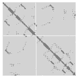
A protein contact map represents the distance between all possible amino acid residue pairs of a three-dimensional protein structure using a binary two-dimensional matrix. For two residues and , the element of the matrix is 1 if the two residues are closer than a predetermined threshold, and 0 otherwise. Various contact definitions have been proposed: The distance between the Cα-Cα atom with threshold 6-12 Å; distance between Cβ-Cβ atoms with threshold 6-12 Å ; and distance between the side-chain centers of mass.
Solvent exposure occurs when a chemical, material, or person comes into contact with a solvent. Chemicals can be dissolved in solvents, materials such as polymers can be broken down chemically by solvents, and people can develop certain ailments from exposure to solvents both organic and inorganic.
In computational biology, protein pKa calculations are used to estimate the pKa values of amino acids as they exist within proteins. These calculations complement the pKa values reported for amino acids in their free state, and are used frequently within the fields of molecular modeling, structural bioinformatics, and computational biology.
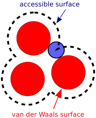
The accessible surface area (ASA) or solvent-accessible surface area (SASA) is the surface area of a biomolecule that is accessible to a solvent. Measurement of ASA is usually described in units of square angstroms. ASA was first described by Lee & Richards in 1971 and is sometimes called the Lee-Richards molecular surface. ASA is typically calculated using the 'rolling ball' algorithm developed by Shrake & Rupley in 1973. This algorithm uses a sphere of a particular radius to 'probe' the surface of the molecule.
In chemistry, a contact number (CN) is a simple solvent exposure measure that measures residue burial in proteins. The definition of CN varies between authors, but is generally defined as the number of either C or C atoms within a sphere around the C or C atom of the residue. The radius of the sphere is typically chosen to be between 8 and 14Å.
The global distance test (GDT), also written as GDT_TS to represent "total score", is a measure of similarity between two protein structures with known amino acid correspondences but different tertiary structures. It is most commonly used to compare the results of protein structure prediction to the experimentally determined structure as measured by X-ray crystallography, protein NMR, or, increasingly, cryoelectron microscopy. The metric was developed by Adam Zemla at Lawrence Livermore National Laboratory and originally implemented in the Local-Global Alignment (LGA) program. It is intended as a more accurate measurement than the common root-mean-square deviation (RMSD) metric - which is sensitive to outlier regions created, for example, by poor modeling of individual loop regions in a structure that is otherwise reasonably accurate. The conventional GDT_TS score is computed over the alpha carbon atoms and is reported as a percentage, ranging from 0 to 100. In general, the higher the GDT_TS score, the more closely a model approximates a given reference structure.
Structural and physical properties of DNA provide important constraints on the binding sites formed on surfaces of DNA-binding proteins. Characteristics of such binding sites may be used for predicting DNA-binding sites from the structural and even sequence properties of unbound proteins. This approach has been successfully implemented for predicting the protein–protein interface. Here, this approach is adopted for predicting DNA-binding sites in DNA-binding proteins. First attempt to use sequence and evolutionary features to predict DNA-binding sites in proteins was made by Ahmad et al. (2004) and Ahmad and Sarai (2005). Some methods use structural information to predict DNA-binding sites and therefore require a three-dimensional structure of the protein, while others use only sequence information and do not require protein structure in order to make a prediction.
FoldX is a protein design algorithm that uses an empirical force field. It can determine the energetic effect of point mutations as well as the interaction energy of protein complexes. FoldX can mutate protein and DNA side chains using a probability-based rotamer library, while exploring alternative conformations of the surrounding side chains.
Computational Resources for Drug Discovery (CRDD) is one of the important silico modules of Open Source for Drug Discovery (OSDD). The CRDD web portal provides computer resources related to drug discovery on a single platform. It provides computational resources for researchers in computer-aided drug design, a discussion forum, and resources to maintain a wiki related to drug discovery, predict inhibitors, and predict the ADME-Tox property of molecules. One of the major objectives of CRDD is to promote open source software in the field of chemoinformatics and pharmacoinformatics.
Residue depth (RD) is a solvent exposure measure that describes to what extent a residue is buried in the protein structure space. It complements the information provided by conventional accessible surface area (ASA).
Triple resonance experiments are a set of multi-dimensional nuclear magnetic resonance spectroscopy (NMR) experiments that link three types of atomic nuclei, most typically consisting of 1H, 15N and 13C. These experiments are often used to assign specific resonance signals to specific atoms in an isotopically-enriched protein. The technique was first described in papers by Ad Bax, Mitsuhiko Ikura and Lewis Kay in 1990, and further experiments were then added to the suite of experiments. Many of these experiments have since become the standard set of experiments used for sequential assignment of NMR resonances in the determination of protein structure by NMR. They are now an integral part of solution NMR study of proteins, and they may also be used in solid-state NMR.

The chemical shift index or CSI is a widely employed technique in protein nuclear magnetic resonance spectroscopy that can be used to display and identify the location as well as the type of protein secondary structure found in proteins using only backbone chemical shift data The technique was invented by David S. Wishart in 1992 for analyzing 1Hα chemical shifts and then later extended by him in 1994 to incorporate 13C backbone shifts. The original CSI method makes use of the fact that 1Hα chemical shifts of amino acid residues in helices tends to be shifted upfield relative to their random coil values and downfield in beta strands. Similar kinds of upfield and downfield trends are also detectable in backbone 13C chemical shifts.
Relative accessible surface area or relative solvent accessibility (RSA) of a protein residue is a measure of residue solvent exposure. It can be calculated by formula:

In biochemistry, a backbone-dependent rotamer library provides the frequencies, mean dihedral angles, and standard deviations of the discrete conformations of the amino acid side chains in proteins as a function of the backbone dihedral angles φ and ψ of the Ramachandran map. By contrast, backbone-independent rotamer libraries express the frequencies and mean dihedral angles for all side chains in proteins, regardless of the backbone conformation of each residue type. Backbone-dependent rotamer libraries have been shown to have significant advantages over backbone-independent rotamer libraries, principally when used as an energy term, by speeding up search times of side-chain packing algorithms used in protein structure prediction and protein design.
