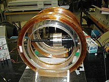
Two circular coil device which creates a homogeneous magnetic field
A Helmholtz coilHelmholtz coil schematic drawing
A Helmholtz coil is a device for producing a region of nearly uniform magnetic field, named after the German physicist Hermann von Helmholtz. It consists of two electromagnets on the same axis, carrying an equal electric current in the same direction. Besides creating magnetic fields, Helmholtz coils are also used in scientific apparatus to cancel external magnetic fields, such as the Earth's magnetic field.
A beam of cathode rays in a vacuum tube bent into a circle by a Helmholtz coil
Description
A Helmholtz pair consists of two identical circular magnetic coils that are placed symmetrically along a common axis, one on each side of the experimental area, and separated by a distance equal to the radius of the coil. Each coil carries an equal electric current in the same direction.[1]
Setting , which is what defines a Helmholtz pair, minimizes the nonuniformity of the field at the center of the coils, in the sense of setting [2] (meaning that the first nonzero derivative is as explained below), but leaves about 7% variation in field strength between the center and the planes of the coils. A slightly larger value of reduces the difference in field between the center and the planes of the coils, at the expense of worsening the field's uniformity in the region near the center, as measured by .[3]
In some applications, a Helmholtz coil is used to cancel out the Earth's magnetic field, producing a region with a magnetic field intensity much closer to zero.[4]
Mathematics
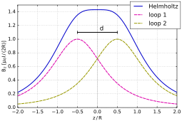
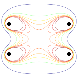
Magnetic field lines in a plane bisecting the current loops. Note the field is approximately uniform in between the coil pair. (In this picture the coils are placed one beside the other: the axis is horizontal.)Magnetic field induction along the axis crossing the center of coils; z=0 is the point in the middle of the distance between coilsContours showing the magnitude of the magnetic field near a coil pair, with one coil at top and the other at bottom. Inside the central "octopus", the field is within 1% of its central value B0. The eight contours are for field magnitudes of 0.5B0, 0.8B0, 0.9B0, 0.95B0, 0.99B0, 1.01B0, 1.05B0, and 1.1B0.
The calculation of the exact magnetic field at any point in space is mathematically complex and involves the study of Bessel functions. Things are simpler along the axis of the coil-pair, and it is convenient to think about the Taylor series expansion of the field strength as a function of , the distance from the central point of the coil-pair along the axis. By symmetry, the odd-order terms in the expansion are zero. By arranging the coils so that the origin is an inflection point for the field strength due to each coil separately, one can guarantee that the order term is also zero, and hence the leading non-constant term is of order . The inflection point for a simple coil is located along the coil axis at a distance from its centre. Thus the locations for the two coils are .
The calculation detailed below gives the exact value of the magnetic field at the center point. If the radius is R, the number of turns in each coil is n and the current through the coils is I, then the magnetic field B at the midpoint between the coils will be given by
is the distance dependent, dimensionless coefficient.
The Helmholtz coils consists of n turns of wire, so the equivalent current in a one-turn coil is n times the current I in the n-turn coil. Substituting nI for I in the above formula gives the field for an n-turn coil:
For , the distance coefficient can be expanded in Taylor series as:
In a Helmholtz pair, the two coils are located at , so the B-field strength at any would be:
The points near the center (halfway between the two coils) have , and the Taylor series of is:
.
Time-varying magnetic field
Most Helmholtz coils use DC (direct) current to produce a static magnetic field. Many applications and experiments require a time-varying magnetic field. These applications include magnetic field susceptibility tests, scientific experiments, and biomedical studies (the interaction between magnetic field and living tissue). The required magnetic fields are usually either pulse or continuous sinewave. The magnetic field frequency range can be anywhere from near DC (0Hz) to many kilohertz or even megahertz (MHz). An AC Helmholtz coil driver is needed to generate the required time-varying magnetic field. The waveform amplifier driver must be able to output high AC current to produce the magnetic field.
Driver voltage and current
Use the above equation in the mathematics section to calculate the coil current for a desired magnetic field, B.
where is the permeability of free space or
= coil current, in amperes,
= coil radius, in meters,
n = number of turns in each coil.
Using a function generator and a high-current waveform amplifier driver to generate high-frequency Helmholtz magnetic field
Then calculate the required Helmholtz coil driver amplifier voltage:[6]
where
I is the peak current,
ω is the angular frequency or ω = 2πf,
L1 and L2 are the inductances of the two Helmholtz coils, and
R1 and R2 are the resistances of the two coils.
High-frequency series resonant
Generating a static magnetic field is relatively easy; the strength of the field is proportional to the current. Generating a high-frequency magnetic field is more challenging. The coils are inductors, and their impedance increases proportionally with frequency. To provide the same field intensity at twice the frequency requires twice the voltage across the coil. Instead of directly driving the coil with a high voltage, a series resonant circuit may be used to provide the high voltage.[7] A series capacitor is added in series with the coils. The capacitance is chosen to resonate the coil at the desired frequency. Only the coils parasitic resistance remains. This method only works at frequencies close to the resonant frequency; to generate the field at other frequencies requires different capacitors. The Helmholtz coil resonant frequency, , and capacitor value, C, are given below.[6]
Anti-Helmholtz coil
When the pair of two electromagnets of a Helmholtz coil carry an equal electric current in the opposite direction, it is known as anti-Helmholtz coil, which creates a region of nearly uniform magnetic field gradient, and is used for creating magnetic traps for atomic physics experiments.
In an anti-Helmholtz pair, the B-field strength at any would be:
The points near the center (halfway between the two coils) have , and the Taylor series of is:
.
Maxwell coils
Helmholtz coils (hoops) on three perpendicular axes used to cancel the Earth's magnetic field inside the vacuum tank in a 1957 electron beam experiment
To improve the uniformity of the field in the space inside the coils, additional coils can be added around the outside. James Clerk Maxwell showed in 1873 that a third larger-diameter coil located midway between the two Helmholtz coils with the coil distance increased from coil radius to can reduce the variance of the field on the axis to zero up to the sixth derivative of position. This is sometimes called a Maxwell coil.
A magnetic bottle has the same structure as Helmholtz coils, but with the magnets separated further apart so that the field expands in the middle, trapping charged particles with the diverging field lines. If one coil is reversed, it produces a cusp trap, which also traps charged particles.[8]
Helmholtz coils were designed and built for the Army Research Laboratory's electromagnetic composite testing laboratory in 1993, for testing of composite materials to low-frequency magnetic fields.[9]
References
↑ Ramsden, Edward (2006). Hall-effect sensors: theory and applications (2nded.). Amsterdam: Elsevier/Newnes. p.195. ISBN978-0-75067934-3.
This page is based on this Wikipedia article Text is available under the CC BY-SA 4.0 license; additional terms may apply. Images, videos and audio are available under their respective licenses.