where the curve has discriminant Then the point has order 3.
To prove that has order 3, note that the tangent to at is the line which intersects with multiplicity 3 at .
Conversely, given a point of order 3 on an elliptic curve both defined over a field one can put the curve into Weierstrass form with so that the tangent at is the line . Then the equation of the curve is with .
To obtain the Hessian curve, it is necessary to do the following transformation:
It is interesting to analyze the group law of the elliptic curve, defining the addition and doubling formulas (because the SPA and DPA attacks are based on the running time of these operations). Furthermore, in this case, we only need to use the same procedure to compute the addition, doubling or subtraction of points to get efficient results, as said above. In general, the group law is defined in the following way: if three points lie in the same line then they sum up to zero. So, by this property, the group laws are different for every curve.
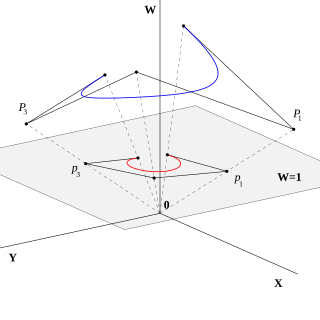
In this case, the correct way is to use the Cauchy-Desboves´ formulas, obtaining the point at infinity θ = (1: −1: 0), that is, the neutral element (the inverse of θ is θ again). Let P = (x1, y1) be a point on the curve. The line contains the point P and the point at infinity θ. Therefore, −P is the third point of the intersection of this line with the curve. Intersecting the elliptic curve with the line, the following condition is obtained
Since is non zero (because D3 is distinct to 1), the x-coordinate of −P is y1 and the y-coordinate of −P is x1 , i.e., or in projective coordinates .
In some application of elliptic curve cryptography and the elliptic curve method of factorization (ECM) it is necessary to compute the scalar multiplications of P, say [n]P for some integern, and they are based on the double-and-add method; these operations need the addition and doubling formulas.
Doubling
Now, if is a point on the elliptic curve, it is possible to define a "doubling" operation using Cauchy-Desboves´ formulae:
Addition
In the same way, for two different points, say and , it is possible to define the addition formula. Let R denote the sum of these points, R = P + Q, then its coordinates are given by:
Algorithms and examples
There is one algorithm that can be used to add two different points or to double; it is given by Joye and Quisquater. Then, the following result gives the possibility the obtain the doubling operation by the addition:
Proposition. Let P = (X,Y,Z) be a point on a Hessian elliptic curve E(K). Then:
(2)
Furthermore, we have (Z:X:Y) ≠ (Y:Z:X).
Finally, contrary to other parameterizations, there is no subtraction to compute the negation of a point. Hence, this addition algorithm can also be used for subtracting two points P = (X1:Y1:Z1) and Q = (X2:Y2:Z2) on a Hessian elliptic curve:
(3)
To sum up, by adapting the order of the inputs according to equation (2) or (3), the addition algorithm presented above can be used indifferently for: Adding 2 (diff.) points, Doubling a point and Subtracting 2 points with only 12 multiplications and 7 auxiliary variables including the 3 result variables. Before the invention of Edwards curves, these results represent the fastest known method for implementing the elliptic curve scalar multiplication towards resistance against side-channel attacks.
For some algorithms protection against side-channel attacks is not necessary. So, for these doublings can be faster. Since there are many algorithms, only the best for the addition and doubling formulas is given here, with one example for each one:
Addition
Let P1 = (X1:Y1:Z1) and P2 = (X2:Y2:Z2) be two points distinct to θ. Assuming that Z1 = Z2 = 1 then the algorithm is given by:
A = X1Y2
B = Y1X2
X3 = BY1-Y2A
Y3 = X1A-BX2
Z3 = Y2X2-X1Y1
The cost needed is 8 multiplications and 3 additions readdition cost of 7 multiplications and 3 additions, depending on the first point.
Example
Given the following points in the curve for d = −1 P1 = (1:0:−1) and P2 = (0:−1:1), then if P3 = P1 + P2 we have:
X3 = 0 − 1 = −1
Y3 = −1−0 = −1
Z3 = 0 − 0 = 0
Then: P3 = (−1:−1:0)
Doubling
Let P = (X1: Y1: Z1) be a point, then the doubling formula is given by:
A = X12
B = Y12
D = A + B
G = (X1 + Y1)2 − D
X3 = (2Y1 − G) × (X1 + A + 1)
Y3 = (G − 2X1) × (Y1 + B + 1)
Z3 = (X1 − Y1) × (G + 2D)
The cost of this algorithm is three multiplications + three squarings + 11 additions + 3×2.
Example
If is a point over the Hessian curve with parameter d = −1, then the coordinates of are given by:
X = (2 . (−1) − 2) (−1 + 1 + 1) = −4
Y = (−4 − 2 . (−1)) ((−1) + 1 + 1) = −2
Z = (−1 − (−1)) ((−4) + 2 . 2) = 0
That is,
Extended coordinates
There is another coordinates system with which a Hessian curve can be represented; these new coordinates are called extended coordinates. They can speed up the addition and doubling. To have more information about operations with the extended coordinates see:
↑ Cauchy-Desbove's Formulae: Hessian-elliptic Curves and Side-Channel Attacks, Marc Joye and Jean-Jacques Quisquarter
Related Research Articles
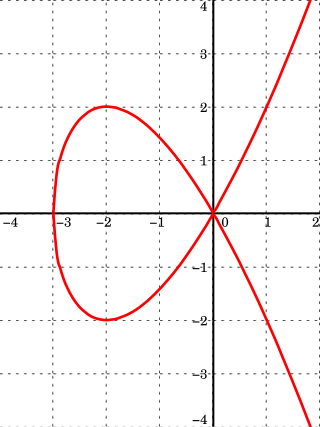
In mathematics, an elliptic curve is a smooth, projective, algebraic curve of genus one, on which there is a specified point O. An elliptic curve is defined over a field K and describes points in K2, the Cartesian product of K with itself. If the field's characteristic is different from 2 and 3, then the curve can be described as a plane algebraic curve which consists of solutions (x, y) for:
In probability theory, a probability density function (PDF), density function, or density of an absolutely continuous random variable, is a function whose value at any given sample in the sample space can be interpreted as providing a relative likelihood that the value of the random variable would be equal to that sample. Probability density is the probability per unit length, in other words, while the absolute likelihood for a continuous random variable to take on any particular value is 0, the value of the PDF at two different samples can be used to infer, in any particular draw of the random variable, how much more likely it is that the random variable would be close to one sample compared to the other sample.
Bresenham's line algorithm is a line drawing algorithm that determines the points of an n-dimensional raster that should be selected in order to form a close approximation to a straight line between two points. It is commonly used to draw line primitives in a bitmap image, as it uses only integer addition, subtraction, and bit shifting, all of which are very cheap operations in historically common computer architectures. It is an incremental error algorithm, and one of the earliest algorithms developed in the field of computer graphics. The extension to the original algorithm may, called midpoint circle algorithm, be used for drawing circles.
The Lenstra elliptic-curve factorization or the elliptic-curve factorization method (ECM) is a fast, sub-exponential running time, algorithm for integer factorization, which employs elliptic curves. For general-purpose factoring, ECM is the third-fastest known factoring method. The second-fastest is the multiple polynomial quadratic sieve, and the fastest is the general number field sieve. The Lenstra elliptic-curve factorization is named after Hendrik Lenstra.
In mathematics, the Laplace operator or Laplacian is a differential operator given by the divergence of the gradient of a scalar function on Euclidean space. It is usually denoted by the symbols , (where is the nabla operator), or . In a Cartesian coordinate system, the Laplacian is given by the sum of second partial derivatives of the function with respect to each independent variable. In other coordinate systems, such as cylindrical and spherical coordinates, the Laplacian also has a useful form. Informally, the Laplacian Δf (p) of a function f at a point p measures by how much the average value of f over small spheres or balls centered at p deviates from f (p).
In linear algebra, two vectors in an inner product space are orthonormal if they are orthogonal unit vectors. A set of vectors form an orthonormal set if all vectors in the set are mutually orthogonal and all of unit length. An orthonormal set which forms a basis is called an orthonormal basis.
In mathematics, homogeneous coordinates or projective coordinates, introduced by August Ferdinand Möbius in his 1827 work Der barycentrische Calcul, are a system of coordinates used in projective geometry, just as Cartesian coordinates are used in Euclidean geometry. They have the advantage that the coordinates of points, including points at infinity, can be represented using finite coordinates. Formulas involving homogeneous coordinates are often simpler and more symmetric than their Cartesian counterparts. Homogeneous coordinates have a range of applications, including computer graphics and 3D computer vision, where they allow affine transformations and, in general, projective transformations to be easily represented by a matrix. They are also used in fundamental elliptic curve cryptography algorithms.
In vector calculus, Green's theorem relates a line integral around a simple closed curve C to a double integral over the plane region D bounded by C. It is the two-dimensional special case of Stokes' theorem.
In mathematics, an affine algebraic plane curve is the zero set of a polynomial in two variables. A projective algebraic plane curve is the zero set in a projective plane of a homogeneous polynomial in three variables. An affine algebraic plane curve can be completed in a projective algebraic plane curve by homogenizing its defining polynomial. Conversely, a projective algebraic plane curve of homogeneous equation h(x, y, t) = 0 can be restricted to the affine algebraic plane curve of equation h(x, y, 1) = 0. These two operations are each inverse to the other; therefore, the phrase algebraic plane curve is often used without specifying explicitly whether it is the affine or the projective case that is considered.
Linear elasticity is a mathematical model of how solid objects deform and become internally stressed due to prescribed loading conditions. It is a simplification of the more general nonlinear theory of elasticity and a branch of continuum mechanics.
In geometry, an incidence relation is a heterogeneous relation that captures the idea being expressed when phrases such as "a point lies on a line" or "a line is contained in a plane" are used. The most basic incidence relation is that between a point, P, and a line, l, sometimes denoted P I l. If P I l the pair (P, l) is called a flag. There are many expressions used in common language to describe incidence (for example, a line passes through a point, a point lies in a plane, etc.) but the term "incidence" is preferred because it does not have the additional connotations that these other terms have, and it can be used in a symmetric manner. Statements such as "line l1 intersects line l2" are also statements about incidence relations, but in this case, it is because this is a shorthand way of saying that "there exists a point P that is incident with both line l1 and line l2". When one type of object can be thought of as a set of the other type of object (viz., a plane is a set of points) then an incidence relation may be viewed as containment.
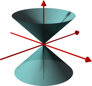
In geometry, a (general) conical surface is the unbounded surface formed by the union of all the straight lines that pass through a fixed point — the apex or vertex — and any point of some fixed space curve — the directrix — that does not contain the apex. Each of those lines is called a generatrix of the surface.
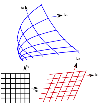
In geometry, curvilinear coordinates are a coordinate system for Euclidean space in which the coordinate lines may be curved. These coordinates may be derived from a set of Cartesian coordinates by using a transformation that is locally invertible at each point. This means that one can convert a point given in a Cartesian coordinate system to its curvilinear coordinates and back. The name curvilinear coordinates, coined by the French mathematician Lamé, derives from the fact that the coordinate surfaces of the curvilinear systems are curved.
In computer graphics, the Liang–Barsky algorithm is a line clipping algorithm. The Liang–Barsky algorithm uses the parametric equation of a line and inequalities describing the range of the clipping window to determine the intersections between the line and the clip window. With these intersections it knows which portion of the line should be drawn. So this algorithm is significantly more efficient than Cohen–Sutherland. The idea of the Liang–Barsky clipping algorithm is to do as much testing as possible before computing line intersections.
In geometry, line coordinates are used to specify the position of a line just as point coordinates are used to specify the position of a point.
In mathematics, the Edwards curves are a family of elliptic curves studied by Harold Edwards in 2007. The concept of elliptic curves over finite fields is widely used in elliptic curve cryptography. Applications of Edwards curves to cryptography were developed by Daniel J. Bernstein and Tanja Lange: they pointed out several advantages of the Edwards form in comparison to the more well known Weierstrass form.
In mathematics, the Jacobi curve is a representation of an elliptic curve different from the usual one defined by the Weierstrass equation. Sometimes it is used in cryptography instead of the Weierstrass form because it can provide a defence against simple and differential power analysis style (SPA) attacks; it is possible, indeed, to use the general addition formula also for doubling a point on an elliptic curve of this form: in this way the two operations become indistinguishable from some side-channel information. The Jacobi curve also offers faster arithmetic compared to the Weierstrass curve.
In mathematics, the Twisted Hessian curve represents a generalization of Hessian curves; it was introduced in elliptic curve cryptography to speed up the addition and doubling formulas and to have strongly unified arithmetic. In some operations, it is close in speed to Edwards curves.
In mathematics, the doubling-oriented Doche–Icart–Kohel curve is a form in which an elliptic curve can be written. It is a special case of Weierstrass form and it is also important in elliptic-curve cryptography because the doubling speeds up considerably. It has been introduced by Christophe Doche, Thomas Icart, and David R. Kohel in Efficient Scalar Multiplication by Isogeny Decompositions.
In algebraic geometry, the twisted Edwards curves are plane models of elliptic curves, a generalisation of Edwards curves introduced by Bernstein, Birkner, Joye, Lange and Peters in 2008. The curve set is named after mathematician Harold M. Edwards. Elliptic curves are important in public key cryptography and twisted Edwards curves are at the heart of an electronic signature scheme called EdDSA that offers high performance while avoiding security problems that have surfaced in other digital signature schemes.
References
Otto Hesse (1844), "Über die Elimination der Variabeln aus drei algebraischen Gleichungen vom zweiten Grade mit zwei Variabeln", Journal für die reine und angewandte Mathematik, 10, pp.68–96
Marc Joye, Jean-Jacques Quisquater (2001). "Hessian Elliptic Curves and Side-Channel Attacks". Cryptographic Hardware and Embedded Systems — CHES 2001. Lecture Notes in Computer Science. Vol.2162. Springer-Verlag Berlin Heidelberg 2001. pp.402–410. doi:10.1007/3-540-44709-1_33. ISBN978-3-540-42521-2.
N. P. Smart (2001). "The Hessian form of an Elliptic Curve". Cryptographic Hardware and Embedded Systems — CHES 2001. Lecture Notes in Computer Science. Vol.2162. Springer-Verlag Berlin Heidelberg 2001. pp.118–125. doi:10.1007/3-540-44709-1_11. ISBN978-3-540-42521-2. S2CID30487134.
This page is based on this Wikipedia article Text is available under the CC BY-SA 4.0 license; additional terms may apply. Images, videos and audio are available under their respective licenses.