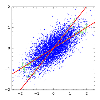
In regression analysis, least squares is a parameter estimation method based on minimizing the sum of the squares of the residuals made in the results of each individual equation.

In probability theory and statistics, the Gumbel distribution is used to model the distribution of the maximum of a number of samples of various distributions.
In probability and statistics, an exponential family is a parametric set of probability distributions of a certain form, specified below. This special form is chosen for mathematical convenience, including the enabling of the user to calculate expectations, covariances using differentiation based on some useful algebraic properties, as well as for generality, as exponential families are in a sense very natural sets of distributions to consider. The term exponential class is sometimes used in place of "exponential family", or the older term Koopman–Darmois family. Sometimes loosely referred to as "the" exponential family, this class of distributions is distinct because they all possess a variety of desirable properties, most importantly the existence of a sufficient statistic.
Empirical Bayes methods are procedures for statistical inference in which the prior probability distribution is estimated from the data. This approach stands in contrast to standard Bayesian methods, for which the prior distribution is fixed before any data are observed. Despite this difference in perspective, empirical Bayes may be viewed as an approximation to a fully Bayesian treatment of a hierarchical model wherein the parameters at the highest level of the hierarchy are set to their most likely values, instead of being integrated out. Empirical Bayes, also known as maximum marginal likelihood, represents a convenient approach for setting hyperparameters, but has been mostly supplanted by fully Bayesian hierarchical analyses since the 2000s with the increasing availability of well-performing computation techniques. It is still commonly used, however, for variational methods in Deep Learning, such as variational autoencoders, where latent variable spaces are high-dimensional.
In statistics, a generalized linear model (GLM) is a flexible generalization of ordinary linear regression. The GLM generalizes linear regression by allowing the linear model to be related to the response variable via a link function and by allowing the magnitude of the variance of each measurement to be a function of its predicted value.

In statistics, nonlinear regression is a form of regression analysis in which observational data are modeled by a function which is a nonlinear combination of the model parameters and depends on one or more independent variables. The data are fitted by a method of successive approximations (iterations).
In statistics, econometrics, epidemiology and related disciplines, the method of instrumental variables (IV) is used to estimate causal relationships when controlled experiments are not feasible or when a treatment is not successfully delivered to every unit in a randomized experiment. Intuitively, IVs are used when an explanatory variable of interest is correlated with the error term (endogenous), in which case ordinary least squares and ANOVA give biased results. A valid instrument induces changes in the explanatory variable but has no independent effect on the dependent variable and is not correlated with the error term, allowing a researcher to uncover the causal effect of the explanatory variable on the dependent variable.

In statistics, ordinary least squares (OLS) is a type of linear least squares method for choosing the unknown parameters in a linear regression model by the principle of least squares: minimizing the sum of the squares of the differences between the observed dependent variable in the input dataset and the output of the (linear) function of the independent variable. Some sources consider OLS to be linear regression.
In statistics, generalized least squares (GLS) is a method used to estimate the unknown parameters in a linear regression model. It is used when there is a non-zero amount of correlation between the residuals in the regression model. GLS is employed to improve statistical efficiency and reduce the risk of drawing erroneous inferences, as compared to conventional least squares and weighted least squares methods. It was first described by Alexander Aitken in 1935.
Multilevel models are statistical models of parameters that vary at more than one level. An example could be a model of student performance that contains measures for individual students as well as measures for classrooms within which the students are grouped. These models can be seen as generalizations of linear models, although they can also extend to non-linear models. These models became much more popular after sufficient computing power and software became available.
In statistics, binomial regression is a regression analysis technique in which the response has a binomial distribution: it is the number of successes in a series of independent Bernoulli trials, where each trial has probability of success . In binomial regression, the probability of a success is related to explanatory variables: the corresponding concept in ordinary regression is to relate the mean value of the unobserved response to explanatory variables.
A mixed model, mixed-effects model or mixed error-component model is a statistical model containing both fixed effects and random effects. These models are useful in a wide variety of disciplines in the physical, biological and social sciences. They are particularly useful in settings where repeated measurements are made on the same statistical units, or where measurements are made on clusters of related statistical units. Mixed models are often preferred over traditional analysis of variance regression models because they don't rely on the independent observations assumption. Further, they have their flexibility in dealing with missing values and uneven spacing of repeated measurements. The Mixed model analysis allows measurements to be explicitly modeled in a wider variety of correlation and variance-covariance avoiding biased estimations structures.
In statistics, identifiability is a property which a model must satisfy for precise inference to be possible. A model is identifiable if it is theoretically possible to learn the true values of this model's underlying parameters after obtaining an infinite number of observations from it. Mathematically, this is equivalent to saying that different values of the parameters must generate different probability distributions of the observable variables. Usually the model is identifiable only under certain technical restrictions, in which case the set of these requirements is called the identification conditions.

In statistics, an errors-in-variables model or a measurement error model is a regression model that accounts for measurement errors in the independent variables. In contrast, standard regression models assume that those regressors have been measured exactly, or observed without error; as such, those models account only for errors in the dependent variables, or responses.
The generalized additive model for location, scale and shape (GAMLSS) is a semiparametric regression model in which a parametric statistical distribution is assumed for the response (target) variable but the parameters of this distribution can vary according to explanatory variables. GAMLSS is a form of supervised machine learning.
In statistics, the variance function is a smooth function that depicts the variance of a random quantity as a function of its mean. The variance function is a measure of heteroscedasticity and plays a large role in many settings of statistical modelling. It is a main ingredient in the generalized linear model framework and a tool used in non-parametric regression, semiparametric regression and functional data analysis. In parametric modeling, variance functions take on a parametric form and explicitly describe the relationship between the variance and the mean of a random quantity. In a non-parametric setting, the variance function is assumed to be a smooth function.
The generalized functional linear model (GFLM) is an extension of the generalized linear model (GLM) that allows one to regress univariate responses of various types on functional predictors, which are mostly random trajectories generated by a square-integrable stochastic processes. Similarly to GLM, a link function relates the expected value of the response variable to a linear predictor, which in case of GFLM is obtained by forming the scalar product of the random predictor function with a smooth parameter function . Functional Linear Regression, Functional Poisson Regression and Functional Binomial Regression, with the important Functional Logistic Regression included, are special cases of GFLM. Applications of GFLM include classification and discrimination of stochastic processes and functional data.
In statistics, linear regression is a model that estimates the linear relationship between a scalar response and one or more explanatory variables. A model with exactly one explanatory variable is a simple linear regression; a model with two or more explanatory variables is a multiple linear regression. This term is distinct from multivariate linear regression, which predicts multiple correlated dependent variables rather than a single dependent variable.
In statistics, the class of vector generalized linear models (VGLMs) was proposed to enlarge the scope of models catered for by generalized linear models (GLMs). In particular, VGLMs allow for response variables outside the classical exponential family and for more than one parameter. Each parameter can be transformed by a link function. The VGLM framework is also large enough to naturally accommodate multiple responses; these are several independent responses each coming from a particular statistical distribution with possibly different parameter values.
Nonlinear mixed-effects models constitute a class of statistical models generalizing linear mixed-effects models. Like linear mixed-effects models, they are particularly useful in settings where there are multiple measurements within the same statistical units or when there are dependencies between measurements on related statistical units. Nonlinear mixed-effects models are applied in many fields including medicine, public health, pharmacology, and ecology.


