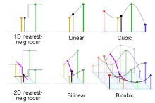
In the mathematical field of numerical analysis, interpolation is a type of estimation, a method of constructing (finding) new data points based on the range of a discrete set of known data points.
In digital signal processing, spatial anti-aliasing is a technique for minimizing the distortion artifacts (aliasing) when representing a high-resolution image at a lower resolution. Anti-aliasing is used in digital photography, computer graphics, digital audio, and many other applications.

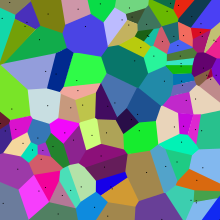
In mathematics, a Voronoi diagram is a partition of a plane into regions close to each of a given set of objects. It can be classified also as a tessellation. In the simplest case, these objects are just finitely many points in the plane. For each seed there is a corresponding region, called a Voronoi cell, consisting of all points of the plane closer to that seed than to any other. The Voronoi diagram of a set of points is dual to that set's Delaunay triangulation.

Nonlinear dimensionality reduction, also known as manifold learning, is any of various related techniques that aim to project high-dimensional data, potentially existing across non-linear manifolds which cannot be adequately captured by linear decomposition methods, onto lower-dimensional latent manifolds, with the goal of either visualizing the data in the low-dimensional space, or learning the mapping itself. The techniques described below can be understood as generalizations of linear decomposition methods used for dimensionality reduction, such as singular value decomposition and principal component analysis.

In scientific visualization and computer graphics, volume rendering is a set of techniques used to display a 2D projection of a 3D discretely sampled data set, typically a 3D scalar field.
In computer graphics, texture filtering or texture smoothing is the method used to determine the texture color for a texture mapped pixel, using the colors of nearby texels.
The scale-invariant feature transform (SIFT) is a computer vision algorithm to detect, describe, and match local features in images, invented by David Lowe in 1999. Applications include object recognition, robotic mapping and navigation, image stitching, 3D modeling, gesture recognition, video tracking, individual identification of wildlife and match moving.

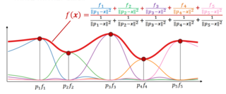
Inverse distance weighting (IDW) is a type of deterministic method for multivariate interpolation with a known scattered set of points. The assigned values to unknown points are calculated with a weighted average of the values available at the known points. This method can also be used to create spatial weights matrices in spatial autocorrelation analyses.

In computer science, a k-d tree is a space-partitioning data structure for organizing points in a k-dimensional space. K-dimensional is that which concerns exactly k orthogonal axes or a space of any number of dimensions. k-d trees are a useful data structure for several applications, such as:
In statistics, the k-nearest neighbors algorithm (k-NN) is a non-parametric supervised learning method. It was first developed by Evelyn Fix and Joseph Hodges in 1951, and later expanded by Thomas Cover. Most often, it is used for classification, as a k-NN classifier, the output of which is a class membership. An object is classified by a plurality vote of its neighbors, with the object being assigned to the class most common among its k nearest neighbors (k is a positive integer, typically small). If k = 1, then the object is simply assigned to the class of that single nearest neighbor.

Marching tetrahedra is an algorithm in the field of computer graphics to render implicit surfaces. It clarifies a minor ambiguity problem of the marching cubes algorithm with some cube configurations. It was originally introduced in 1991.
Demosaicing, also known as color reconstruction, is a digital image processing algorithm used to reconstruct a full color image from the incomplete color samples output from an image sensor overlaid with a color filter array (CFA) such as a Bayer filter. It is also known as CFA interpolation or debayering.
In computer graphics, marching squares is an algorithm that generates contours for a two-dimensional scalar field. A similar method can be used to contour 2D triangle meshes.
Nearest neighbor search (NNS), as a form of proximity search, is the optimization problem of finding the point in a given set that is closest to a given point. Closeness is typically expressed in terms of a dissimilarity function: the less similar the objects, the larger the function values.
In numerical analysis, multivariate interpolation is interpolation on functions of more than one variable ; when the variates are spatial coordinates, it is also known as spatial interpolation.
Region growing is a simple region-based image segmentation method. It is also classified as a pixel-based image segmentation method since it involves the selection of initial seed points.

The Point Cloud Library (PCL) is an open-source library of algorithms for point cloud processing tasks and 3D geometry processing, such as occur in three-dimensional computer vision. The library contains algorithms for filtering, feature estimation, surface reconstruction, 3D registration, model fitting, object recognition, and segmentation. Each module is implemented as a smaller library that can be compiled separately. PCL has its own data format for storing point clouds - PCD, but also allows datasets to be loaded and saved in many other formats. It is written in C++ and released under the BSD license.
In computer science, a ball tree, balltree or metric tree, is a space partitioning data structure for organizing points in a multi-dimensional space. A ball tree partitions data points into a nested set of balls. The resulting data structure has characteristics that make it useful for a number of applications, most notably nearest neighbor search.
This is a glossary of terms relating to computer graphics.


