
In mathematics, the discrete Fourier transform (DFT) converts a finite sequence of equally-spaced samples of a function into a same-length sequence of equally-spaced samples of the discrete-time Fourier transform (DTFT), which is a complex-valued function of frequency. The interval at which the DTFT is sampled is the reciprocal of the duration of the input sequence. An inverse DFT (IDFT) is a Fourier series, using the DTFT samples as coefficients of complex sinusoids at the corresponding DTFT frequencies. It has the same sample-values as the original input sequence. The DFT is therefore said to be a frequency domain representation of the original input sequence. If the original sequence spans all the non-zero values of a function, its DTFT is continuous, and the DFT provides discrete samples of one cycle. If the original sequence is one cycle of a periodic function, the DFT provides all the non-zero values of one DTFT cycle.

Frequency, most often measured in hertz, is the number of occurrences of a repeating event per unit of time. It is also occasionally referred to as temporal frequency for clarity and to distinguish it from spatial frequency. Ordinary frequency is related to angular frequency by a factor of 2π. The period is the interval of time between events, so the period is the reciprocal of the frequency: f = 1/T.

The Nyquist–Shannon sampling theorem is an essential principle for digital signal processing linking the frequency range of a signal and the sample rate required to avoid a type of distortion called aliasing. The theorem states that the sample rate must be at least twice the bandwidth of the signal to avoid aliasing. In practice, it is used to select band-limiting filters to keep aliasing below an acceptable amount when an analog signal is sampled or when sample rates are changed within a digital signal processing function.

In signal processing, the Nyquist rate, named after Harry Nyquist, is a value equal to twice the highest frequency (bandwidth) of a given function or signal. When the function is digitized at a higher sample rate, the resulting discrete-time sequence is said to be free of the distortion known as aliasing. Conversely, for a given sample-rate the corresponding Nyquist frequency in Hz is one-half the sample-rate. Note that the Nyquist rate is a property of a continuous-time signal, whereas Nyquist frequency is a property of a discrete-time system.
A low-pass filter is a filter that passes signals with a frequency lower than a selected cutoff frequency and attenuates signals with frequencies higher than the cutoff frequency. The exact frequency response of the filter depends on the filter design. The filter is sometimes called a high-cut filter, or treble-cut filter in audio applications. A low-pass filter is the complement of a high-pass filter.

In signal processing and related disciplines, aliasing is the overlapping of frequency components resulting from a sample rate below the Nyquist rate. This overlap results in distortion or artifacts when the signal is reconstructed from samples which causes the reconstructed signal to differ from the original continuous signal. Aliasing that occurs in signals sampled in time, for instance in digital audio or the stroboscopic effect, is referred to as temporal aliasing. Aliasing in spatially sampled signals is referred to as spatial aliasing.
In mathematics and signal processing, the Z-transform converts a discrete-time signal, which is a sequence of real or complex numbers, into a complex valued frequency-domain representation.

In physics, angular frequency, also called angular speed and angular rate, is a scalar measure of the angle rate or the temporal rate of change of the phase argument of a sinusoidal waveform or sine function . Angular frequency is the magnitude of the pseudovector quantity angular velocity.
A sine wave, sinusoidal wave, or sinusoid is a periodic wave whose waveform (shape) is the trigonometric sine function. In mechanics, as a linear motion over time, this is simple harmonic motion; as rotation, it corresponds to uniform circular motion. Sine waves occur often in physics, including wind waves, sound waves, and light waves, such as monochromatic radiation. In engineering, signal processing, and mathematics, Fourier analysis decomposes general functions into a sum of sine waves of various frequencies, relative phases, and magnitudes.

The short-time Fourier transform (STFT), is a Fourier-related transform used to determine the sinusoidal frequency and phase content of local sections of a signal as it changes over time. In practice, the procedure for computing STFTs is to divide a longer time signal into shorter segments of equal length and then compute the Fourier transform separately on each shorter segment. This reveals the Fourier spectrum on each shorter segment. One then usually plots the changing spectra as a function of time, known as a spectrogram or waterfall plot, such as commonly used in software defined radio (SDR) based spectrum displays. Full bandwidth displays covering the whole range of an SDR commonly use fast Fourier transforms (FFTs) with 2^24 points on desktop computers.
In signal processing, a finite impulse response (FIR) filter is a filter whose impulse response is of finite duration, because it settles to zero in finite time. This is in contrast to infinite impulse response (IIR) filters, which may have internal feedback and may continue to respond indefinitely.
Rotational frequency, also known as rotational speed or rate of rotation, is the frequency of rotation of an object around an axis. Its SI unit is the reciprocal seconds (s−1); other common units of measurement include the hertz (Hz), cycles per second (cps), and revolutions per minute (rpm).
In applied mathematics, a DFT matrix is an expression of a discrete Fourier transform (DFT) as a transformation matrix, which can be applied to a signal through matrix multiplication.

In mathematics, the concept of signed frequency can indicate both the rate and sense of rotation; it can be as simple as a wheel rotating clockwise or counterclockwise. The rate is expressed in units such as revolutions per second (hertz) or radian/second.
In mathematics, the discrete-time Fourier transform (DTFT) is a form of Fourier analysis that is applicable to a sequence of discrete values.
In signal processing, linear phase is a property of a filter where the phase response of the filter is a linear function of frequency. The result is that all frequency components of the input signal are shifted in time by the same constant amount, which is referred to as the group delay. Consequently, there is no phase distortion due to the time delay of frequencies relative to one another.

In mathematics, a Dirac comb is a periodic function with the formula

In digital signal processing, upsampling, expansion, and interpolation are terms associated with the process of resampling in a multi-rate digital signal processing system. Upsampling can be synonymous with expansion, or it can describe an entire process of expansion and filtering (interpolation). When upsampling is performed on a sequence of samples of a signal or other continuous function, it produces an approximation of the sequence that would have been obtained by sampling the signal at a higher rate. For example, if compact disc audio at 44,100 samples/second is upsampled by a factor of 5/4, the resulting sample-rate is 55,125.
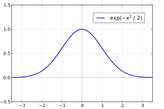
The Gabor transform, named after Dennis Gabor, is a special case of the short-time Fourier transform. It is used to determine the sinusoidal frequency and phase content of local sections of a signal as it changes over time. The function to be transformed is first multiplied by a Gaussian function, which can be regarded as a window function, and the resulting function is then transformed with a Fourier transform to derive the time-frequency analysis. The window function means that the signal near the time being analyzed will have higher weight. The Gabor transform of a signal x(t) is defined by this formula:
Impulse invariance is a technique for designing discrete-time infinite-impulse-response (IIR) filters from continuous-time filters in which the impulse response of the continuous-time system is sampled to produce the impulse response of the discrete-time system. The frequency response of the discrete-time system will be a sum of shifted copies of the frequency response of the continuous-time system; if the continuous-time system is approximately band-limited to a frequency less than the Nyquist frequency of the sampling, then the frequency response of the discrete-time system will be approximately equal to it for frequencies below the Nyquist frequency.


