Order of accuracy

Last updated May 08, 2023

In numerical analysis, order of accuracy quantifies the rate of convergence of a numerical approximation of a differential equation to the exact solution. Consider $u$ , the exact solution to a differential equation in an appropriate normed space $(V,||\ ||)$ . Consider a numerical approximation $u_{h}$ , where $h$ is a parameter characterizing the approximation, such as the step size in a finite difference scheme or the diameter of the cells in a finite element method. The numerical solution $u_{h}$ is said to be $n$ th-order accurate if the error $E(h):=||u-u_{h}||$ is proportional to the step-size $h$ to the $n$ th power:^[1]

E(h)=||u-u_{h}||\leq Ch^{n}

where the constant $C$ is independent of $h$ and usually depends on the solution $u$ .^[2] Using the big O notation an $n$ th-order accurate numerical method is notated as

||u-u_{h}||=O(h^{n})

This definition is strictly dependent on the norm used in the space; the choice of such norm is fundamental to estimate the rate of convergence and, in general, all numerical errors correctly.

The size of the error of a first-order accurate approximation is directly proportional to $h$ . Partial differential equations which vary over both time and space are said to be accurate to order $n$ in time and to order $m$ in space.^[3]

Related Research Articles

<span class="mw-page-title-main">Numerical analysis</span> Study of algorithms using numerical approximation

Numerical analysis is the study of algorithms that use numerical approximation for the problems of mathematical analysis. It is the study of numerical methods that attempt at finding approximate solutions of problems rather than the exact ones. Numerical analysis finds application in all fields of engineering and the physical sciences, and in the 21st century also the life and social sciences, medicine, business and even the arts. Current growth in computing power has enabled the use of more complex numerical analysis, providing detailed and realistic mathematical models in science and engineering. Examples of numerical analysis include: ordinary differential equations as found in celestial mechanics, numerical linear algebra in data analysis, and stochastic differential equations and Markov chains for simulating living cells in medicine and biology.

In the mathematical subfield of numerical analysis, numerical stability is a generally desirable property of numerical algorithms. The precise definition of stability depends on the context. One is numerical linear algebra and the other is algorithms for solving ordinary and partial differential equations by discrete approximation.

Numerical methods for ordinary differential equations are methods used to find numerical approximations to the solutions of ordinary differential equations (ODEs). Their use is also known as "numerical integration", although this term can also refer to the computation of integrals.

Numerical methods for partial differential equations is the branch of numerical analysis that studies the numerical solution of partial differential equations (PDEs).

In mathematics, the convergence condition by Courant–Friedrichs–Lewy is a necessary condition for convergence while solving certain partial differential equations numerically. It arises in the numerical analysis of explicit time integration schemes, when these are used for the numerical solution. As a consequence, the time step must be less than a certain time in many explicit time-marching computer simulations, otherwise the simulation produces incorrect results. The condition is named after Richard Courant, Kurt Friedrichs, and Hans Lewy who described it in their 1928 paper.

In mathematics, in the area of numerical analysis, Galerkin methods are named after the Soviet mathematician Boris Galerkin. They convert a continuous operator problem, such as a differential equation, commonly in a weak formulation, to a discrete problem by applying linear constraints determined by finite sets of basis functions.

In mathematics and computational science, the Euler method is a first-order numerical procedure for solving ordinary differential equations (ODEs) with a given initial value. It is the most basic explicit method for numerical integration of ordinary differential equations and is the simplest Runge–Kutta method. The Euler method is named after Leonhard Euler, who first proposed it in his book Institutionum calculi integralis.

<span class="mw-page-title-main">Computational electromagnetics</span> Branch of physics

Computational electromagnetics (CEM), computational electrodynamics or electromagnetic modeling is the process of modeling the interaction of electromagnetic fields with physical objects and the environment.

In numerical analysis and computational fluid dynamics, Godunov's scheme is a conservative numerical scheme, suggested by S. K. Godunov in 1959, for solving partial differential equations. One can think of this method as a conservative finite-volume method which solves exact, or approximate Riemann problems at each inter-cell boundary. In its basic form, Godunov's method is first order accurate in both space and time, yet can be used as a base scheme for developing higher-order methods.

In numerical analysis, finite-difference methods (FDM) are a class of numerical techniques for solving differential equations by approximating derivatives with finite differences. Both the spatial domain and time interval are discretized, or broken into a finite number of steps, and the value of the solution at these discrete points is approximated by solving algebraic equations containing finite differences and values from nearby points.

In the numerical solution of partial differential equations, a topic in mathematics, the spectral element method (SEM) is a formulation of the finite element method (FEM) that uses high degree piecewise polynomials as basis functions. The spectral element method was introduced in a 1984 paper by A. T. Patera. Although Patera is credited with development of the method, his work was a rediscovery of an existing method

The patch test in the finite element method is a simple indicator of the quality of a finite element, developed by Bruce Irons. The patch test uses a partial differential equation on a domain consisting from several elements set up so that the exact solution is known and can be reproduced, in principle, with zero error. Typically, in mechanics, the prescribed exact solution consists of displacements that vary as piecewise linear functions in space. The elements pass the patch test if the finite element solution is the same as the exact solution.

In computational physics, the term upwind scheme typically refers to a class of numerical discretization methods for solving hyperbolic partial differential equations, in which so-called upstream variables are used to calculate the derivatives in a flow field. That is, derivatives are estimated using a set of data points biased to be more "upwind" of the query point, with respect to the direction of the flow. Historically, the origin of upwind methods can be traced back to the work of Courant, Isaacson, and Rees who proposed the CIR method.

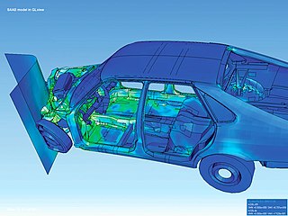
The finite element method (FEM) is a popular method for numerically solving differential equations arising in engineering and mathematical modeling. Typical problem areas of interest include the traditional fields of structural analysis, heat transfer, fluid flow, mass transport, and electromagnetic potential.

hp-FEM is a general version of the finite element method (FEM), a numerical method for solving partial differential equations based on piecewise-polynomial approximations that employs elements of variable size (h) and polynomial degree (p). The origins of hp-FEM date back to the pioneering work of Barna A. Szabó and Ivo Babuška who discovered that the finite element method converges exponentially fast when the mesh is refined using a suitable combination of h-refinements (dividing elements into smaller ones) and p-refinements. The exponential convergence makes the method very attractive compared to most other finite element methods, which only converge with an algebraic rate. The exponential convergence of hp-FEM was not only predicted theoretically, but also observed by numerous independent researchers.

The Kansa method is a computer method used to solve partial differential equations. Its main advantage is it is very easy to understand and program on a computer. It is much less complicated than the finite element method. Another advantage is it works well on multi variable problems. The finite element method is complicated when working with more than 3 space variables and time.

False diffusion is a type of error observed when the upwind scheme is used to approximate the convection term in convection–diffusion equations. The more accurate central difference scheme can be used for the convection term, but for grids with cell Peclet number more than 2, the central difference scheme is unstable and the simpler upwind scheme is often used. The resulting error from the upwind differencing scheme has a diffusion-like appearance in two- or three-dimensional co-ordinate systems and is referred as "false diffusion". False-diffusion errors in numerical solutions of convection-diffusion problems, in two- and three-dimensions, arise from the numerical approximations of the convection term in the conservation equations. Over the past 20 years many numerical techniques have been developed to solve convection-diffusion equations and none are problem-free, but false diffusion is one of the most serious problems and a major topic of controversy and confusion among numerical analysts.

Fluid motion is governed by the Navier–Stokes equations, a set of coupled and nonlinear partial differential equations derived from the basic laws of conservation of mass, momentum and energy. The unknowns are usually the flow velocity, the pressure and density and temperature. The analytical solution of this equation is impossible hence scientists resort to laboratory experiments in such situations. The answers delivered are, however, usually qualitatively different since dynamical and geometric similitude are difficult to enforce simultaneously between the lab experiment and the prototype. Furthermore, the design and construction of these experiments can be difficult, particularly for stratified rotating flows. Computational fluid dynamics (CFD) is an additional tool in the arsenal of scientists. In its early days CFD was often controversial, as it involved additional approximation to the governing equations and raised additional (legitimate) issues. Nowadays CFD is an established discipline alongside theoretical and experimental methods. This position is in large part due to the exponential growth of computer power which has allowed us to tackle ever larger and more complex problems.

<span class="mw-page-title-main">Gradient discretisation method</span>

In numerical mathematics, the gradient discretisation method (GDM) is a framework which contains classical and recent numerical schemes for diffusion problems of various kinds: linear or non-linear, steady-state or time-dependent. The schemes may be conforming or non-conforming, and may rely on very general polygonal or polyhedral meshes.

References

↑ LeVeque, Randall J (2006). Finite Difference Methods for Differential Equations. University of Washington. pp. 3–5. CiteSeerX 10.1.1.111.1693 .
↑ Ciarliet, Philippe J (1978). The Finite Element Method for Elliptic Problems. Elsevier. pp. 105–106. doi:10.1137/1.9780898719208. ISBN 978-0-89871-514-9.
↑ Strikwerda, John C (2004). Finite Difference Schemes and Partial Differential Equations (2 ed.). pp. 62–66. ISBN 978-0-898716-39-9.

This applied mathematics-related article is a stub. You can help Wikipedia by expanding it.

This page is based on this Wikipedia article
Text is available under the CC BY-SA 4.0 license; additional terms may apply.
Images, videos and audio are available under their respective licenses.

[LeVeque-1] LeVeque, Randall J (2006). Finite Difference Methods for Differential Equations. University of Washington. pp. 3–5. CiteSeerX 10.1.1.111.1693 .

[2] Ciarliet, Philippe J (1978). The Finite Element Method for Elliptic Problems. Elsevier. pp. 105–106. doi:10.1137/1.9780898719208. ISBN 978-0-89871-514-9.

[Strikwerda-3] Strikwerda, John C (2004). Finite Difference Schemes and Partial Differential Equations (2 ed.). pp. 62–66. ISBN 978-0-898716-39-9.

[1]

[2]

[3]