
In electrical engineering, a transmission line is a specialized cable or other structure designed to conduct electromagnetic waves in a contained manner. The term applies when the conductors are long enough that the wave nature of the transmission must be taken into account. This applies especially to radio-frequency engineering because the short wavelengths mean that wave phenomena arise over very short distances. However, the theory of transmission lines was historically developed to explain phenomena on very long telegraph lines, especially submarine telegraph cables.
Unit quaternions, known as versors, provide a convenient mathematical notation for representing spatial orientations and rotations of elements in three dimensional space. Specifically, they encode information about an axis-angle rotation about an arbitrary axis. Rotation and orientation quaternions have applications in computer graphics, computer vision, robotics, navigation, molecular dynamics, flight dynamics, orbital mechanics of satellites, and crystallographic texture analysis.

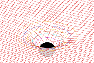
In the general theory of relativity, the Einstein field equations relate the geometry of spacetime to the distribution of matter within it.

The Lotka–Volterra equations, also known as the predator–prey equations, are a pair of first-order nonlinear differential equations, frequently used to describe the dynamics of biological systems in which two species interact, one as a predator and the other as prey. The populations change through time according to the pair of equations:
In differential geometry, the Cotton tensor on a (pseudo)-Riemannian manifold of dimension n is a third-order tensor concomitant of the metric. The vanishing of the Cotton tensor for n = 3 is necessary and sufficient condition for the manifold to be conformally flat. By contrast, in dimensions n ≥ 4, the vanishing of the Cotton tensor is necessary but not sufficient for the metric to be conformally flat; instead, the corresponding necessary and sufficient condition in these higher dimensions is the vanishing of the Weyl tensor, while the Cotton tensor just becomes a constant times the divergence of the Weyl tensor. For n < 3 the Cotton tensor is identically zero. The concept is named after Émile Cotton.
The rigid rotor is a mechanical model of rotating systems. An arbitrary rigid rotor is a 3-dimensional rigid object, such as a top. To orient such an object in space requires three angles, known as Euler angles. A special rigid rotor is the linear rotor requiring only two angles to describe, for example of a diatomic molecule. More general molecules are 3-dimensional, such as water, ammonia, or methane.
In differential geometry, the four-gradient is the four-vector analogue of the gradient from vector calculus.
In differential geometry, a tensor density or relative tensor is a generalization of the tensor field concept. A tensor density transforms as a tensor field when passing from one coordinate system to another, except that it is additionally multiplied or weighted by a power W of the Jacobian determinant of the coordinate transition function or its absolute value. A distinction is made among (authentic) tensor densities, pseudotensor densities, even tensor densities and odd tensor densities. Sometimes tensor densities with a negative weight W are called tensor capacity. A tensor density can also be regarded as a section of the tensor product of a tensor bundle with a density bundle.
When studying and formulating Albert Einstein's theory of general relativity, various mathematical structures and techniques are utilized. The main tools used in this geometrical theory of gravitation are tensor fields defined on a Lorentzian manifold representing spacetime. This article is a general description of the mathematics of general relativity.

In electromagnetism, the electromagnetic tensor or electromagnetic field tensor is a mathematical object that describes the electromagnetic field in spacetime. The field tensor was first used after the four-dimensional tensor formulation of special relativity was introduced by Hermann Minkowski. The tensor allows related physical laws to be written very concisely.
In physics, Larmor precession is the precession of the magnetic moment of an object about an external magnetic field. The phenomenon is conceptually similar to the precession of a tilted classical gyroscope in an external torque-exerting gravitational field. Objects with a magnetic moment also have angular momentum and effective internal electric current proportional to their angular momentum; these include electrons, protons, other fermions, many atomic and nuclear systems, as well as classical macroscopic systems. The external magnetic field exerts a torque on the magnetic moment,
The covariant formulation of classical electromagnetism refers to ways of writing the laws of classical electromagnetism in a form that is manifestly invariant under Lorentz transformations, in the formalism of special relativity using rectilinear inertial coordinate systems. These expressions both make it simple to prove that the laws of classical electromagnetism take the same form in any inertial coordinate system, and also provide a way to translate the fields and forces from one frame to another. However, this is not as general as Maxwell's equations in curved spacetime or non-rectilinear coordinate systems.
In physics, Maxwell's equations in curved spacetime govern the dynamics of the electromagnetic field in curved spacetime or where one uses an arbitrary coordinate system. These equations can be viewed as a generalization of the vacuum Maxwell's equations which are normally formulated in the local coordinates of flat spacetime. But because general relativity dictates that the presence of electromagnetic fields induce curvature in spacetime, Maxwell's equations in flat spacetime should be viewed as a convenient approximation.
There are various mathematical descriptions of the electromagnetic field that are used in the study of electromagnetism, one of the four fundamental interactions of nature. In this article, several approaches are discussed, although the equations are in terms of electric and magnetic fields, potentials, and charges with currents, generally speaking.
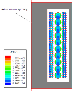
In a conductor carrying alternating current, if currents are flowing through one or more other nearby conductors, such as within a closely wound coil of wire, the distribution of current within the first conductor will be constrained to smaller regions. The resulting current crowding is termed the proximity effect. This crowding gives an increase in the effective resistance of the circuit, which increases with frequency.
The theory of special relativity plays an important role in the modern theory of classical electromagnetism. It gives formulas for how electromagnetic objects, in particular the electric and magnetic fields, are altered under a Lorentz transformation from one inertial frame of reference to another. It sheds light on the relationship between electricity and magnetism, showing that frame of reference determines if an observation follows electrostatic or magnetic laws. It motivates a compact and convenient notation for the laws of electromagnetism, namely the "manifestly covariant" tensor form.

In general relativity, a point mass deflects a light ray with impact parameter by an angle approximately equal to
In continuum mechanics, a compatible deformation tensor field in a body is that unique tensor field that is obtained when the body is subjected to a continuous, single-valued, displacement field. Compatibility is the study of the conditions under which such a displacement field can be guaranteed. Compatibility conditions are particular cases of integrability conditions and were first derived for linear elasticity by Barré de Saint-Venant in 1864 and proved rigorously by Beltrami in 1886.
A frequency-selective surface (FSS) is any thin, repetitive surface designed to reflect, transmit or absorb electromagnetic fields based on the frequency of the field. In this sense, an FSS is a type of optical filter or metal-mesh optical filters in which the filtering is accomplished by virtue of the regular, periodic pattern on the surface of the FSS. Though not explicitly mentioned in the name, FSS's also have properties which vary with incidence angle and polarization as well - these are unavoidable consequences of the way in which FSS's are constructed. Frequency-selective surfaces have been most commonly used in the radio frequency region of the electromagnetic spectrum and find use in applications as diverse as the aforementioned microwave oven, antenna radomes and modern metamaterials. Sometimes frequency selective surfaces are referred to simply as periodic surfaces and are a 2-dimensional analog of the new periodic volumes known as photonic crystals.
In theoretical physics, the dual graviton is a hypothetical elementary particle that is a dual of the graviton under electric-magnetic duality, as an S-duality, predicted by some formulations of supergravity in eleven dimensions.


