Related Research Articles
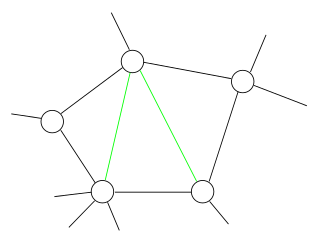
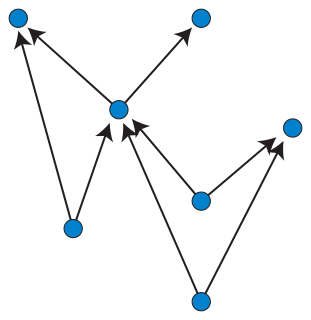
In graph theory, a planar graph is a graph that can be embedded in the plane, i.e., it can be drawn on the plane in such a way that its edges intersect only at their endpoints. In other words, it can be drawn in such a way that no edges cross each other. Such a drawing is called a plane graph or planar embedding of the graph. A plane graph can be defined as a planar graph with a mapping from every node to a point on a plane, and from every edge to a plane curve on that plane, such that the extreme points of each curve are the points mapped from its end nodes, and all curves are disjoint except on their extreme points.

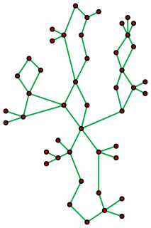
Graph drawing is an area of mathematics and computer science combining methods from geometric graph theory and information visualization to derive two-dimensional depictions of graphs arising from applications such as social network analysis, cartography, linguistics, and bioinformatics.
In graph theory, an undirected graph H is called a minor of the graph G if H can be formed from G by deleting edges and vertices and by contracting edges.
In the mathematical area of graph theory, a chordal graph is one in which all cycles of four or more vertices have a chord, which is an edge that is not part of the cycle but connects two vertices of the cycle. Equivalently, every induced cycle in the graph should have exactly three vertices. The chordal graphs may also be characterized as the graphs that have perfect elimination orderings, as the graphs in which each minimal separator is a clique, and as the intersection graphs of subtrees of a tree. They are sometimes also called rigid circuit graphs or triangulated graphs.
In graph theory, a path decomposition of a graph G is, informally, a representation of G as a "thickened" path graph, and the pathwidth of G is a number that measures how much the path was thickened to form G. More formally, a path-decomposition is a sequence of subsets of vertices of G such that the endpoints of each edge appear in one of the subsets and such that each vertex appears in a contiguous subsequence of the subsets, and the pathwidth is one less than the size of the largest set in such a decomposition. Pathwidth is also known as interval thickness, vertex separation number, or node searching number.
In graph theory, a cactus is a connected graph in which any two simple cycles have at most one vertex in common. Equivalently, it is a connected graph in which every edge belongs to at most one simple cycle, or in which every block is an edge or a cycle.

In graph theory, a branch of mathematics, the triconnected components of a biconnected graph are a system of smaller graphs that describe all of the 2-vertex cuts in the graph. An SPQR tree is a tree data structure used in computer science, and more specifically graph algorithms, to represent the triconnected components of a graph. The SPQR tree of a graph may be constructed in linear time and has several applications in dynamic graph algorithms and graph drawing.
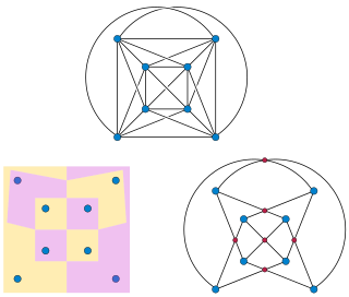
In graph theory, the planarity testing problem is the algorithmic problem of testing whether a given graph is a planar graph. This is a well-studied problem in computer science for which many practical algorithms have emerged, many taking advantage of novel data structures. Most of these methods operate in O(n) time, where n is the number of edges in the graph, which is asymptotically optimal. Rather than just being a single Boolean value, the output of a planarity testing algorithm may be a planar graph embedding, if the graph is planar, or an obstacle to planarity such as a Kuratowski subgraph if it is not.
In graph theory, a branch of discrete mathematics, a distance-hereditary graph is a graph in which the distances in any connected induced subgraph are the same as they are in the original graph. Thus, any induced subgraph inherits the distances of the larger graph.

In graph theory, a branch of mathematics, an apex graph is a graph that can be made planar by the removal of a single vertex. The deleted vertex is called an apex of the graph. It is an apex, not the apex because an apex graph may have more than one apex; for example, in the minimal nonplanar graphs K5 or K3,3, every vertex is an apex. The apex graphs include graphs that are themselves planar, in which case again every vertex is an apex. The null graph is also counted as an apex graph even though it has no vertex to remove.

Layered graph drawing or hierarchical graph drawing is a type of graph drawing in which the vertices of a directed graph are drawn in horizontal rows or layers with the edges generally directed downwards. It is also known as Sugiyama-style graph drawing after Kozo Sugiyama, who first developed this drawing style.

In graph drawing, the angular resolution of a drawing of a graph is the sharpest angle formed by any two edges that meet at a common vertex of the drawing.
In topological graph theory, a 1-planar graph is a graph that can be drawn in the Euclidean plane in such a way that each edge has at most one crossing point, where it crosses a single additional edge. If a 1-planar graph, one of the most natural generalizations of planar graphs, is drawn that way, the drawing is called a 1-plane graph or 1-planar embedding of the graph.
In graph drawing, an upward planar drawing of a directed acyclic graph is an embedding of the graph into the Euclidean plane, in which the edges are represented as non-crossing monotonic upwards curves. That is, the curve representing each edge should have the property that every horizontal line intersects it in at most one point, and no two edges may intersect except at a shared endpoint. In this sense, it is the ideal case for layered graph drawing, a style of graph drawing in which edges are monotonic curves that may cross, but in which crossings are to be minimized.
In graph drawing, the area used by a drawing is a commonly used way of measuring its quality.
In graph drawing styles that represent the edges of a graph by polylines, it is desirable to minimize the number of bends per edge or the total number of bends in a drawing. Bend minimization is the algorithmic problem of finding a drawing that minimizes these quantities.
In graph theory, a family of graphs is said to have bounded expansion if all of its shallow minors are sparse graphs. Many natural families of sparse graphs have bounded expansion. A closely related but stronger property, polynomial expansion, is equivalent to the existence of separator theorems for these families. Families with these properties have efficient algorithms for problems including the subgraph isomorphism problem and model checking for the first order theory of graphs.
Simultaneous embedding is a technique in graph drawing and information visualization for visualizing two or more different graphs on the same or overlapping sets of labeled vertices, while avoiding crossings within both graphs. Crossings between an edge of one graph and an edge of the other graph are allowed.
In graph theory, a branch of mathematics, a map graph is an undirected graph formed as the intersection graph of finitely many simply connected and internally disjoint regions of the Euclidean plane. The map graphs include the planar graphs, but are more general. Any number of regions can meet at a common corner, and when they do the map graph will contain a clique connecting the corresponding vertices, unlike planar graphs in which the largest cliques have only four vertices. Another example of a map graph is the king's graph, a map graph of the squares of the chessboard connecting pairs of squares between which the chess king can move.

In combinatorial optimization, the matroid parity problem is a problem of finding the largest independent set of paired elements in a matroid. The problem was formulated by Lawler (1976) as a common generalization of graph matching and matroid intersection. It is also known as polymatroid matching, or the matchoid problem.
References
- 1 2 3 4 5 6 7 8 9 Buchheim, Christoph; Chimani, Markus; Gutwenger, Carsten; Jünger, Michael; Mutzel, Petra (2014), "Crossings and planarization", in Tamassia, Roberto (ed.), Handbook of Graph Drawing and Visualization, Discrete Mathematics and its Applications (Boca Raton), CRC Press, Boca Raton, Florida.
- 1 2 3 4 Di Battista, Giuseppe; Eades, Peter; Tamassia, Roberto; Tollis, Ioannis G. (1998), Graph Drawing: Algorithms for the Visualization of Graphs (1st ed.), Prentice Hall, pp. 215–218, ISBN 0133016153 .
- 1 2 Chimani, Markus (2008), Computing Crossing Numbers (PDF), Ph.D. dissertation, Technical University of Dortmund, Section 4.3.1, archived from the original (PDF) on 2015-11-16.
- 1 2 Călinescu, Gruia; Fernandes, Cristina G.; Finkler, Ulrich; Karloff, Howard (1998), "A better approximation algorithm for finding planar subgraphs", Journal of Algorithms, 27 (2): 269–302, doi:10.1006/jagm.1997.0920, MR 1622397 .
- ↑ Kawarabayashi, Ken-ichi; Reed, Bruce (2007), "Computing crossing number in linear time", Proceedings of the Thirty-ninth Annual ACM Symposium on Theory of Computing (STOC '07), pp. 382–390, doi:10.1145/1250790.1250848, MR 2402463 .
- ↑ Jünger, M.; Mutzel, P. (1996), "Maximum planar subgraphs and nice embeddings: practical layout tools", Algorithmica, 16 (1): 33–59, doi:10.1007/s004539900036, MR 1394493 .
- ↑ Weisstein, Eric W. "Graph Skewness". MathWorld .
- ↑ Kawarabayashi, Ken-ichi (2009), "Planarity allowing few error vertices in linear time", 50th Annual IEEE Symposium on Foundations of Computer Science (FOCS '09) (PDF), pp. 639–648, doi:10.1109/FOCS.2009.45, MR 2648441 .
- ↑ Edwards, Keith; Farr, Graham (2002), "An algorithm for finding large induced planar subgraphs", Graph Drawing: 9th International Symposium, GD 2001 Vienna, Austria, September 23–26, 2001, Revised Papers, Lecture Notes in Comp. Sci., 2265, Springer, pp. 75–80, doi: 10.1007/3-540-45848-4_6 , MR 1962420 .
- ↑ Gutwenger, Carsten; Mutzel, Petra; Weiskircher, René (2005), "Inserting an edge into a planar graph", Algorithmica, 41 (4): 289–308, doi:10.1007/s00453-004-1128-8, MR 2122529 .