Digital image processing is the use of a digital computer to process digital images through an algorithm. As a subcategory or field of digital signal processing, digital image processing has many advantages over analog image processing. It allows a much wider range of algorithms to be applied to the input data and can avoid problems such as the build-up of noise and distortion during processing. Since images are defined over two dimensions, digital image processing may be modeled in the form of multidimensional systems. The generation and development of digital image processing are mainly affected by three factors: first, the development of computers; second, the development of mathematics ; and third, the demand for a wide range of applications in environment, agriculture, military, industry and medical science has increased.
Levinson recursion or Levinson–Durbin recursion is a procedure in linear algebra to recursively calculate the solution to an equation involving a Toeplitz matrix. The algorithm runs in Θ(n2) time, which is a strong improvement over Gauss–Jordan elimination, which runs in Θ(n3).
Edge detection includes a variety of mathematical methods that aim at identifying edges, defined as curves in a digital image at which the image brightness changes sharply or, more formally, has discontinuities. The same problem of finding discontinuities in one-dimensional signals is known as step detection and the problem of finding signal discontinuities over time is known as change detection. Edge detection is a fundamental tool in image processing, machine vision and computer vision, particularly in the areas of feature detection and feature extraction.
Branch and bound is a method for solving optimization problems by breaking them down into smaller sub-problems and using a bounding function to eliminate sub-problems that cannot contain the optimal solution. It is an algorithm design paradigm for discrete and combinatorial optimization problems, as well as mathematical optimization. A branch-and-bound algorithm consists of a systematic enumeration of candidate solutions by means of state space search: the set of candidate solutions is thought of as forming a rooted tree with the full set at the root. The algorithm explores branches of this tree, which represent subsets of the solution set. Before enumerating the candidate solutions of a branch, the branch is checked against upper and lower estimated bounds on the optimal solution, and is discarded if it cannot produce a better solution than the best one found so far by the algorithm.

The Sobel operator, sometimes called the Sobel–Feldman operator or Sobel filter, is used in image processing and computer vision, particularly within edge detection algorithms where it creates an image emphasising edges. It is named after Irwin Sobel and Gary M. Feldman, colleagues at the Stanford Artificial Intelligence Laboratory (SAIL). Sobel and Feldman presented the idea of an "Isotropic 3 × 3 Image Gradient Operator" at a talk at SAIL in 1968. Technically, it is a discrete differentiation operator, computing an approximation of the gradient of the image intensity function. At each point in the image, the result of the Sobel–Feldman operator is either the corresponding gradient vector or the norm of this vector. The Sobel–Feldman operator is based on convolving the image with a small, separable, and integer-valued filter in the horizontal and vertical directions and is therefore relatively inexpensive in terms of computations. On the other hand, the gradient approximation that it produces is relatively crude, in particular for high-frequency variations in the image.

An octree is a tree data structure in which each internal node has exactly eight children. Octrees are most often used to partition a three-dimensional space by recursively subdividing it into eight octants. Octrees are the three-dimensional analog of quadtrees. The word is derived from oct + tree. Octrees are often used in 3D graphics and 3D game engines.
Mehrotra's predictor–corrector method in optimization is a specific interior point method for linear programming. It was proposed in 1989 by Sanjay Mehrotra.

In shape analysis, skeleton of a shape is a thin version of that shape that is equidistant to its boundaries. The skeleton usually emphasizes geometrical and topological properties of the shape, such as its connectivity, topology, length, direction, and width. Together with the distance of its points to the shape boundary, the skeleton can also serve as a representation of the shape.
The Prewitt operator is used in image processing, particularly within edge detection algorithms. Technically, it is a discrete differentiation operator, computing an approximation of the gradient of the image intensity function. At each point in the image, the result of the Prewitt operator is either the corresponding gradient vector or the norm of this vector. The Prewitt operator is based on convolving the image with a small, separable, and integer valued filter in horizontal and vertical directions and is therefore relatively inexpensive in terms of computations like Sobel and Kayyali operators. On the other hand, the gradient approximation which it produces is relatively crude, in particular for high frequency variations in the image. The Prewitt operator was developed by Judith M. S. Prewitt.
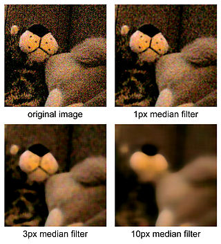
The median filter is a non-linear digital filtering technique, often used to remove noise from an image, signal, and video. Such noise reduction is a typical pre-processing step to improve the results of later processing. Median filtering is very widely used in digital image processing because, under certain conditions, it preserves edges while removing noise, also having applications in signal processing.
In numerical analysis, Bairstow's method is an efficient algorithm for finding the roots of a real polynomial of arbitrary degree. The algorithm first appeared in the appendix of the 1920 book Applied Aerodynamics by Leonard Bairstow. The algorithm finds the roots in complex conjugate pairs using only real arithmetic.
In computer vision, the Lucas–Kanade method is a widely used differential method for optical flow estimation developed by Bruce D. Lucas and Takeo Kanade. It assumes that the flow is essentially constant in a local neighbourhood of the pixel under consideration, and solves the basic optical flow equations for all the pixels in that neighbourhood, by the least squares criterion.
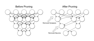
Pruning is a data compression technique in machine learning and search algorithms that reduces the size of decision trees by removing sections of the tree that are non-critical and redundant to classify instances. Pruning reduces the complexity of the final classifier, and hence improves predictive accuracy by the reduction of overfitting.
Sequential quadratic programming (SQP) is an iterative method for constrained nonlinear optimization which may be considered a quasi-Newton method. SQP methods are used on mathematical problems for which the objective function and the constraints are twice continuously differentiable, but not necessarily convex.
Lehmer's GCD algorithm, named after Derrick Henry Lehmer, is a fast GCD algorithm, an improvement on the simpler but slower Euclidean algorithm. It is mainly used for big integers that have a representation as a string of digits relative to some chosen numeral system base, say β = 1000 or β = 232.
In linear algebra, eigendecomposition is the factorization of a matrix into a canonical form, whereby the matrix is represented in terms of its eigenvalues and eigenvectors. Only diagonalizable matrices can be factorized in this way. When the matrix being factorized is a normal or real symmetric matrix, the decomposition is called "spectral decomposition", derived from the spectral theorem.
In digital image processing, morphological skeleton is a skeleton representation of a shape or binary image, computed by means of morphological operators.
In image processing, a kernel, convolution matrix, or mask is a small matrix used for blurring, sharpening, embossing, edge detection, and more. This is accomplished by doing a convolution between the kernel and an image. Or more simply, when each pixel in the output image is a function of the nearby pixels in the input image, the kernel is that function.
Chessboards arise frequently in computer vision theory and practice because their highly structured geometry is well-suited for algorithmic detection and processing. The appearance of chessboards in computer vision can be divided into two main areas: camera calibration and feature extraction. This article provides a unified discussion of the role that chessboards play in the canonical methods from these two areas, including references to the seminal literature, examples, and pointers to software implementations.
Discrete Skeleton Evolution (DSE) describes an iterative approach to reducing a morphological or topological skeleton. It is a form of pruning in that it removes noisy or redundant branches (spurs) generated by the skeletonization process, while preserving information-rich "trunk" segments. The value assigned to individual branches varies from algorithm to algorithm, with the general goal being to convey the features of interest of the original contour with a few carefully chosen lines. Usually, clarity for human vision is valued as well. DSE algorithms are distinguished by complex, recursive decision-making processes with high computational requirements. Pruning methods such as by structuring element (SE) convolution and the Hough transform are general purpose algorithms which quickly pass through an image and eliminate all branches shorter than a given threshold. DSE methods are most applicable when detail retention and contour reconstruction are valued.


