The likelihood function describes the joint probability of the observed data as a function of the parameters of the chosen statistical model. For each specific parameter value in the parameter space, the likelihood function therefore assigns a probabilistic prediction to the observed data . Since it is essentially the product of sampling densities, the likelihood generally encapsulates both the data-generating process as well as the missing-data mechanism that produced the observed sample.
In statistics, naive Bayes classifiers are a family of simple "probabilistic classifiers" based on applying Bayes' theorem with strong (naive) independence assumptions between the features. They are among the simplest Bayesian network models, but coupled with kernel density estimation, they can achieve high accuracy levels.
In statistics, maximum likelihood estimation (MLE) is a method of estimating the parameters of an assumed probability distribution, given some observed data. This is achieved by maximizing a likelihood function so that, under the assumed statistical model, the observed data is most probable. The point in the parameter space that maximizes the likelihood function is called the maximum likelihood estimate. The logic of maximum likelihood is both intuitive and flexible, and as such the method has become a dominant means of statistical inference.
In statistics, a statistic is sufficient with respect to a statistical model and its associated unknown parameter if "no other statistic that can be calculated from the same sample provides any additional information as to the value of the parameter". In particular, a statistic is sufficient for a family of probability distributions if the sample from which it is calculated gives no additional information than the statistic, as to which of those probability distributions is the sampling distribution.
A Bayesian network is a probabilistic graphical model that represents a set of variables and their conditional dependencies via a directed acyclic graph (DAG). Bayesian networks are ideal for taking an event that occurred and predicting the likelihood that any one of several possible known causes was the contributing factor. For example, a Bayesian network could represent the probabilistic relationships between diseases and symptoms. Given symptoms, the network can be used to compute the probabilities of the presence of various diseases.

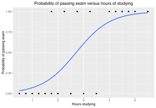
In statistics, the (binary) logistic model is a statistical model that models the probability of one event taking place by having the log-odds for the event be a linear combination of one or more independent variables ("predictors"). In regression analysis, logistic regression is estimating the parameters of a logistic model. Formally, in binary logistic regression there is a single binary dependent variable, coded by a indicator variable, where the two values are labeled "0" and "1", while the independent variables can each be a binary variable or a continuous variable. The corresponding probability of the value labeled "1" can vary between 0 and 1, hence the labeling; the function that converts log-odds to probability is the logistic function, hence the name. The unit of measurement for the log-odds scale is called a logit, from logistic unit, hence the alternative names. See § Background and § Definition for formal mathematics, and § Example for a worked example.
In probability and statistics, an exponential family is a parametric set of probability distributions of a certain form, specified below. This special form is chosen for mathematical convenience, based on some useful algebraic properties, as well as for generality, as exponential families are in a sense very natural sets of distributions to consider. The term exponential class is sometimes used in place of "exponential family", or the older term Koopman–Darmois family. The terms "distribution" and "family" are often used loosely: specifically, an exponential family is a set of distributions, where the specific distribution varies with the parameter; however, a parametric family of distributions is often referred to as "a distribution", and the set of all exponential families is sometimes loosely referred to as "the" exponential family. They are distinct because they possess a variety of desirable properties, most importantly the existence of a sufficient statistic.

In statistics, an expectation–maximization (EM) algorithm is an iterative method to find (local) maximum likelihood or maximum a posteriori (MAP) estimates of parameters in statistical models, where the model depends on unobserved latent variables. The EM iteration alternates between performing an expectation (E) step, which creates a function for the expectation of the log-likelihood evaluated using the current estimate for the parameters, and a maximization (M) step, which computes parameters maximizing the expected log-likelihood found on the E step. These parameter-estimates are then used to determine the distribution of the latent variables in the next E step.
In information geometry, the Fisher information metric is a particular Riemannian metric which can be defined on a smooth statistical manifold, i.e., a smooth manifold whose points are probability measures defined on a common probability space. It can be used to calculate the informational difference between measurements.
In statistics, Gibbs sampling or a Gibbs sampler is a Markov chain Monte Carlo (MCMC) algorithm for obtaining a sequence of observations which are approximated from a specified multivariate probability distribution, when direct sampling is difficult. This sequence can be used to approximate the joint distribution ; to approximate the marginal distribution of one of the variables, or some subset of the variables ; or to compute an integral. Typically, some of the variables correspond to observations whose values are known, and hence do not need to be sampled.
In statistics, the score is the gradient of the log-likelihood function with respect to the parameter vector. Evaluated at a particular point of the parameter vector, the score indicates the steepness of the log-likelihood function and thereby the sensitivity to infinitesimal changes to the parameter values. If the log-likelihood function is continuous over the parameter space, the score will vanish at a local maximum or minimum; this fact is used in maximum likelihood estimation to find the parameter values that maximize the likelihood function.
In statistics, a generalized linear model (GLM) is a flexible generalization of ordinary linear regression. The GLM generalizes linear regression by allowing the linear model to be related to the response variable via a link function and by allowing the magnitude of the variance of each measurement to be a function of its predicted value.
In statistics, a marginal likelihood function, or integrated likelihood, is a likelihood function in which some parameter variables have been marginalized. In the context of Bayesian statistics, it may also be referred to as the evidence or model evidence.

In probability and statistics, the Dirichlet distribution, often denoted , is a family of continuous multivariate probability distributions parameterized by a vector of positive reals. It is a multivariate generalization of the beta distribution, hence its alternative name of multivariate beta distribution (MBD). Dirichlet distributions are commonly used as prior distributions in Bayesian statistics, and in fact the Dirichlet distribution is the conjugate prior of the categorical distribution and multinomial distribution.
Variational Bayesian methods are a family of techniques for approximating intractable integrals arising in Bayesian inference and machine learning. They are typically used in complex statistical models consisting of observed variables as well as unknown parameters and latent variables, with various sorts of relationships among the three types of random variables, as might be described by a graphical model. As typical in Bayesian inference, the parameters and latent variables are grouped together as "unobserved variables". Variational Bayesian methods are primarily used for two purposes:
- To provide an analytical approximation to the posterior probability of the unobserved variables, in order to do statistical inference over these variables.
- To derive a lower bound for the marginal likelihood of the observed data. This is typically used for performing model selection, the general idea being that a higher marginal likelihood for a given model indicates a better fit of the data by that model and hence a greater probability that the model in question was the one that generated the data.
In statistics, the Bayesian information criterion (BIC) or Schwarz information criterion is a criterion for model selection among a finite set of models; models with lower BIC are generally preferred. It is based, in part, on the likelihood function and it is closely related to the Akaike information criterion (AIC).
In statistics, Poisson regression is a generalized linear model form of regression analysis used to model count data and contingency tables. Poisson regression assumes the response variable Y has a Poisson distribution, and assumes the logarithm of its expected value can be modeled by a linear combination of unknown parameters. A Poisson regression model is sometimes known as a log-linear model, especially when used to model contingency tables.
In statistics, binomial regression is a regression analysis technique in which the response has a binomial distribution: it is the number of successes in a series of independent Bernoulli trials, where each trial has probability of success . In binomial regression, the probability of a success is related to explanatory variables: the corresponding concept in ordinary regression is to relate the mean value of the unobserved response to explanatory variables.
In statistics, the observed information, or observed Fisher information, is the negative of the second derivative of the "log-likelihood". It is a sample-based version of the Fisher information.

In probability theory and statistics, the generalized chi-squared distribution is the distribution of a quadratic form of a multinormal variable, or a linear combination of different normal variables and squares of normal variables. Equivalently, it is also a linear sum of independent noncentral chi-square variables and a normal variable. There are several other such generalizations for which the same term is sometimes used; some of them are special cases of the family discussed here, for example the gamma distribution.


