Rule of three (statistics)

Last updated October 26, 2023

In statistical analysis, the rule of three states that if a certain event did not occur in a sample with $n$ subjects, the interval from 0 to 3/ $n$ is a 95% confidence interval for the rate of occurrences in the population. When $n$ is greater than 30, this is a good approximation of results from more sensitive tests. For example, a pain-relief drug is tested on 1500 human subjects, and no adverse event is recorded. From the rule of three, it can be concluded with 95% confidence that fewer than 1 person in 500 (or 3/1500) will experience an adverse event. By symmetry, for only successes, the 95% confidence interval is [1−3/ $n$ ,1].

The rule is useful in the interpretation of clinical trials generally, particularly in phase II and phase III where often there are limitations in duration or statistical power. The rule of three applies well beyond medical research, to any trial done $n$ times. If 300 parachutes are randomly tested and all open successfully, then it is concluded with 95% confidence that fewer than 1 in 100 parachutes with the same characteristics (3/300) will fail.^[1]

Derivation

A 95% confidence interval is sought for the probability p of an event occurring for any randomly selected single individual in a population, given that it has not been observed to occur in n Bernoulli trials. Denoting the number of events by X, we therefore wish to find the values of the parameter p of a binomial distribution that give Pr(X = 0) ≤ 0.05. The rule can then be derived^[2] either from the Poisson approximation to the binomial distribution, or from the formula (1−p)ⁿ for the probability of zero events in the binomial distribution. In the latter case, the edge of the confidence interval is given by Pr(X = 0) = 0.05 and hence (1−p)ⁿ = .05 so n ln(1–p) = ln .05 ≈ −2.996. Rounding the latter to −3 and using the approximation, for p close to 0, that ln(1−p) ≈ −p (Taylor's formula), we obtain the interval's boundary 3/n.

By a similar argument, the numerator values of 3.51, 4.61, and 5.3 may be used for the 97%, 99%, and 99.5% confidence intervals, respectively, and in general the upper end of the confidence interval can be given as ${\frac {-\ln(\alpha )}{n}}$ , where $1-\alpha$ is the desired confidence level.

Extension

The Vysochanskij–Petunin inequality shows that the rule of three holds for unimodal distributions with finite variance beyond just the binomial distribution, and gives a way to change the factor 3 if a different confidence is desired. Chebyshev's inequality removes the assumption of unimodality at the price of a higher multiplier (about 4.5 for 95% confidence). Cantelli's inequality is the one-tailed version of Chebyshev's inequality.

Notes

↑ There are other meanings of the term "rule of three" in mathematics, and a further distinct meaning within statistics:
A century and a half ago Charles Darwin said he had "no Faith in anything short of actual measurement and the Rule of Three," by which he appeared to mean the peak of arithmetical accomplishment in a nineteenth-century gentleman, solving for $x$ in "6 is to 3 as 9 is to $x$ ." Some decades later, in the early 1900s, Karl Pearson shifted the meaning of the rule of three – "take 3σ [three standard deviations] as definitely significant" – and claimed it for his new journal of significance testing, Biometrika. Even Darwin late in life seems to have fallen into the confusion. (Ziliak and McCloskey, 2008, p. 26; parenthetic gloss in original)
↑ "Professor Mean" (2010) "Confidence interval with zero events", The Children's Mercy Hospital. Retrieved 2013-01-01.

Related Research Articles

In probability theory and statistics, the binomial distribution with parameters n and p is the discrete probability distribution of the number of successes in a sequence of n independent experiments, each asking a yes–no question, and each with its own Boolean-valued outcome: success or failure. A single success/failure experiment is also called a Bernoulli trial or Bernoulli experiment, and a sequence of outcomes is called a Bernoulli process; for a single trial, i.e., n = 1, the binomial distribution is a Bernoulli distribution. The binomial distribution is the basis for the popular binomial test of statistical significance.

In probability theory and statistics, a probability distribution is the mathematical function that gives the probabilities of occurrence of different possible outcomes for an experiment. It is a mathematical description of a random phenomenon in terms of its sample space and the probabilities of events.

In probability theory and statistics, the chi-squared distribution with $degrees of freedom is the distribution of a sum of the squares of independent standard normal random variables. The chi-squared distribution is a special case of the gamma distribution and is one of the most widely used probability distributions in inferential statistics, notably in hypothesis testing and in construction of confidence intervals. This distribution is sometimes called the central chi-squared distribution, a special case of the more general noncentral chi-squared distribution.$

In probability theory, Chebyshev's inequality guarantees that, for a wide class of probability distributions, no more than a certain fraction of values can be more than a certain distance from the mean. Specifically, no more than 1/k² of the distribution's values can be k or more standard deviations away from the mean. The rule is often called Chebyshev's theorem, about the range of standard deviations around the mean, in statistics. The inequality has great utility because it can be applied to any probability distribution in which the mean and variance are defined. For example, it can be used to prove the weak law of large numbers.

In statistics, point estimation involves the use of sample data to calculate a single value which is to serve as a "best guess" or "best estimate" of an unknown population parameter. More formally, it is the application of a point estimator to the data to obtain a point estimate.

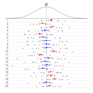
In frequentist statistics, a confidence interval (CI) is a range of estimates for an unknown parameter. A confidence interval is computed at a designated confidence level; the 95% confidence level is most common, but other levels, such as 90% or 99%, are sometimes used. The confidence level, degree of confidence or confidence coefficient represents the long-run proportion of CIs that theoretically contain the true value of the parameter; this is tantamount to the nominal coverage probability. For example, out of all intervals computed at the 95% level, 95% of them should contain the parameter's true value.

In probability theory, the Vysochanskij–Petunin inequality gives a lower bound for the probability that a random variable with finite variance lies within a certain number of standard deviations of the variable's mean, or equivalently an upper bound for the probability that it lies further away. The sole restrictions on the distribution are that it be unimodal and have finite variance.

In mathematics, unimodality means possessing a unique mode. More generally, unimodality means there is only a single highest value, somehow defined, of some mathematical object.

This glossary of statistics and probability is a list of definitions of terms and concepts used in the mathematical sciences of statistics and probability, their sub-disciplines, and related fields. For additional related terms, see Glossary of mathematics and Glossary of experimental design.

In Bayesian statistics, a credible interval is an interval within which an unobserved parameter value falls with a particular probability. It is an interval in the domain of a posterior probability distribution or a predictive distribution. The generalisation to multivariate problems is the credible region.

In statistics, a binomial proportion confidence interval is a confidence interval for the probability of success calculated from the outcome of a series of success–failure experiments. In other words, a binomial proportion confidence interval is an interval estimate of a success probability p when only the number of experiments n and the number of successes n_S are known.

In the theory of probability and statistics, the Dvoretzky–Kiefer–Wolfowitz–Massart inequality bounds how close an empirically determined distribution function will be to the distribution function from which the empirical samples are drawn. It is named after Aryeh Dvoretzky, Jack Kiefer, and Jacob Wolfowitz, who in 1956 proved the inequality

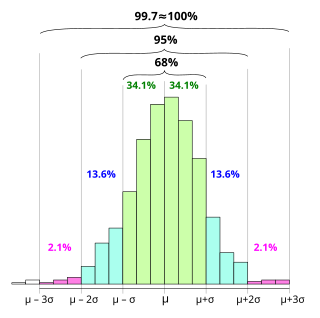
In statistics, the 68–95–99.7 rule, also known as the empirical rule, is a shorthand used to remember the percentage of values that lie within an interval estimate in a normal distribution: 68%, 95%, and 99.7% of the values lie within one, two, and three standard deviations of the mean, respectively.

In probability theory and statistics, the index of dispersion, dispersion index,coefficient of dispersion,relative variance, or variance-to-mean ratio (VMR), like the coefficient of variation, is a normalized measure of the dispersion of a probability distribution: it is a measure used to quantify whether a set of observed occurrences are clustered or dispersed compared to a standard statistical model.

In probability theory, Gauss's inequality gives an upper bound on the probability that a unimodal random variable lies more than any given distance from its mode.

In probability theory and statistics, the Poisson distribution is a discrete probability distribution that expresses the probability of a given number of events occurring in a fixed interval of time or space if these events occur with a known constant mean rate and independently of the time since the last event. It is named after French mathematician Siméon Denis Poisson. The Poisson distribution can also be used for the number of events in other specified interval types such as distance, area, or volume. It plays an important role for discrete-stable distributions.

In statistics and probability theory, the nonparametric skew is a statistic occasionally used with random variables that take real values. It is a measure of the skewness of a random variable's distribution—that is, the distribution's tendency to "lean" to one side or the other of the mean. Its calculation does not require any knowledge of the form of the underlying distribution—hence the name nonparametric. It has some desirable properties: it is zero for any symmetric distribution; it is unaffected by a scale shift; and it reveals either left- or right-skewness equally well. In some statistical samples it has been shown to be less powerful than the usual measures of skewness in detecting departures of the population from normality.

In statistics, cumulative distribution function (CDF)-based nonparametric confidence intervals are a general class of confidence intervals around statistical functionals of a distribution. To calculate these confidence intervals, all that is required is an independently and identically distributed (iid) sample from the distribution and known bounds on the support of the distribution. The latter requirement simply means that all the nonzero probability mass of the distribution must be contained in some known interval $.$

References

Eypasch, Ernst; Rolf Lefering; C. K. Kum; Hans Troidl (1995). "Probability of adverse events that have not yet occurred: A statistical reminder". BMJ. 311 (7005): 619–620. doi:10.1136/bmj.311.7005.619. PMC 2550668 . PMID 7663258.
Hanley, J. A.; A. Lippman-Hand (1983). "If nothing goes wrong, is everything alright?". JAMA. 249 (13): 1743–5. doi:10.1001/jama.1983.03330370053031. PMID 6827763. S2CID 44723518.

Ziliak, S. T.; D. N. McCloskey (2008). The cult of statistical significance: How the standard error costs us jobs, justice, and lives. University of Michigan Press. ISBN 0472050079

This page is based on this Wikipedia article
Text is available under the CC BY-SA 4.0 license; additional terms may apply.
Images, videos and audio are available under their respective licenses.

[1] There are other meanings of the term "rule of three" in mathematics, and a further distinct meaning within statistics:
A century and a half ago Charles Darwin said he had "no Faith in anything short of actual measurement and the Rule of Three," by which he appeared to mean the peak of arithmetical accomplishment in a nineteenth-century gentleman, solving for $x$ in "6 is to 3 as 9 is to $x$ ." Some decades later, in the early 1900s, Karl Pearson shifted the meaning of the rule of three – "take 3σ [three standard deviations] as definitely significant" – and claimed it for his new journal of significance testing, Biometrika. Even Darwin late in life seems to have fallen into the confusion. (Ziliak and McCloskey, 2008, p. 26; parenthetic gloss in original)

[2] "Professor Mean" (2010) "Confidence interval with zero events", The Children's Mercy Hospital. Retrieved 2013-01-01.

[1]

[2]